Doing mathematics with R: Regression analysis in R
 Linear regression in general
We have looked at the linear regression by a straight line in the case where measurement data are described as best as possible through a straight line. It is only important that the parameters to be estimated occur linearly in the formula.
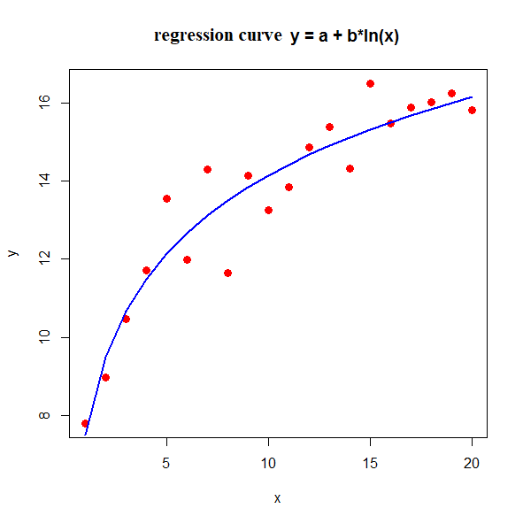
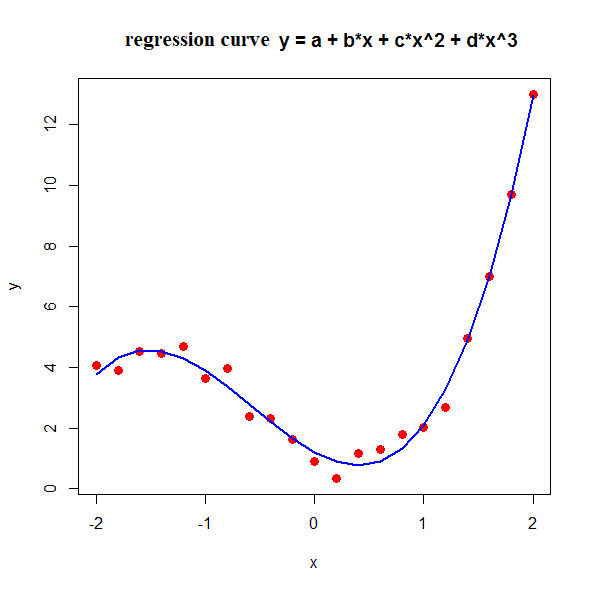
For example, you may also approximate data via a formula such as \(y= \beta_0+\beta_1\cdot \ln(x)\) or allow multiple parameters as in \(y= \beta_0+\beta_1 x + \beta_2 x^2+\beta_3 x^3\). The randomised examples below illustrate this.
y = a + b ln(x)
The R script below produces the diagram shown below.
ln <- function(x) {
  value <- log(x, base=exp(1))
  return(value)
}

# generate random data with noise
x <- seq(from=1, to=20, by=1)
a <- runif(1, min=1, max=10)
b <- runif(1, min=0, max=5)
y <- a+ b*ln(x) + rnorm(20, mean=0, sd=1)

# linear regression
fit <- lm(formula = y ~ ln(x))

# visualisation of data + regression curve
plot(x, y, type = "p", pch = 16, col = "red", cex = 1.3,
     main = "regression curve y = a + b*ln(x)"))
lines(x, predict(fit), type="l", col="blue", lwd=2)

y = a + b·x + c·x² + d·x³
The following R script generates the displayed plot. In this script, the function definition is a linear combination of the constant function \(1\), \(x\), \(x^2\) en \(x^3\), The latter two dependencies are specified using an "as is" construction, denoted as I(x^2) en I(x^3), to ensure that arithmetic operations are correctly interpreted. Alternatively, we could have used poly(x, 3, raw=TRUE).
x <- seq(from=-2, to=2, by=0.2)
b0 <- runif(1, min=1, max=4)
b1 <- runif(1, min=-2, max=2)
b2 <- runif(1, min=1, max=2)
y <- b0 + b1*x + b2*x^2 + x^3 + rnorm(21, mean=0, sd=0.5)

# linear regression
fit <- lm(formula = y ~ 1 + x + I(x^2) + I(x^3))

# visualitation of data + regression curve
plot(x, y, type = "p", pch = 16, col = "red", cex = 1.3,
     main = "regression curve y = a + b*x + c*x^2 + d*x^3")
lines(x, predict(fit), type="l", col="blue", lwd=2)


