We speak of nonlinear regression as soon as model parameters in a regression model do not occur linearly in the regression equation. Below we provide an overview of commonly used nonlinear models in the life sciences context; you may also come across them under other naming conventions.
\[\begin{array}{|c|c|c|} \hline \textbf{model} & \textbf{formula} & \textbf{remark} \\ \hline\\
\text{generalised} & y= \beta_1e^{\beta_2t}+\delta & y(0)=\beta_1+\delta,\\
\text{exponential growth model} & & \delta\text{ is horizontal asymptote} \\ \\ \hline\\
\text{generalised} & y= \beta_1\left(1-e^{-\beta_2(t-\delta)}\right) & y(\delta)=0,\\
\text{Mitscherlich growth model} & & \beta_1\text{ is horizontal asymptote}\\ \\ \hline\\
\text{generalised} & y=\dfrac{\beta_1}{1+\beta_2e^{\beta_3t}}+\delta & y(0)=\dfrac{\beta_1}{1+\beta_2}+\delta,\\
\text{logistic growth model} & & \beta_1+\delta\text{ is horizontal asymptote}\\ \\ \hline\\
\text{Gompertz growth model} & y=\beta_1e^{-\beta_2\e^{-\beta_3t}} & \beta_1\text{ is horizontal asymptote}\\ \\ \hline\\
\text{generalised} & y=\beta_1e^{-\beta_2t}+ \beta_3e^{-\beta_4t}+\delta & \delta\text{ is horizontal asymptote} \\
\text{bi-exponentiel growth model} & & \\ \\ \hline\\
\text{Michaelis-Menten model} & y=\dfrac{\beta_1 x}{\beta_2+x} & \beta_1\text{ is horizontal asymptote}\\ \\ \hline \\
\text{Hill model} & y=\dfrac{\beta_1 x^\gamma}{\beta_2+x^\gamma} & \beta_1\text{ is horizontal asymptote}\\ \\ \hline
\end{array}\]
There are three ways to perform a regression analysis of a nonlinear model:
- Transformation to a linear model;
- Approximation by a linear model (linearisation);
- Nonlinear regression via iterative methods such as the Levenberg-Marquardt method or the Gauss-Newton method.
An example of transformation to a linear model is the exponential growth model \[y=\beta_1e^{\beta_2t}\tiny.\] By transformation with the natural logarithm we get rid of the exponentiation: \[\ln(y)=\ln(\beta_1) +\beta_2t\tiny.\] We have now converted the model equation to a linear regression equation of \(\ln(y)\) versus \(t\).
The multiplication model \(y=\beta_0t^{\beta_1}\) and the S-curve model \(y=e^{\beta_0+\beta_1/t}\) are other examples of regression models that are intrinsically linear because they can be written to a linear model by transformation using the natural logarithm.
The Michaelis-Menten equation \[y=\dfrac{\beta_1 x}{\beta_2+x}\] can be rewritten as \[\frac{1}{y}=\frac{\beta_2}{\beta_1}\cdot\frac{1}{x}+\frac{1}{\beta_1}\] and this implies a linear relationship between \(\dfrac{1}{y}\) and \(\dfrac{1}{x}\).
You can use the nls command (nonlinear least squares) in R to carry out a nonlinear regression using iterative methods. If all goes well, you only have to specify the formula of the model and an iterative solution method is automatically selected, but in many practical cases you have to provide suitable starting values of parameters and specify the method to be used.
The following randomised example illustrates the case where you do not have to specify starting values in a nonlinear regression because the method used converges to an answer anyway (R also reports the choice of starting values).
# generate parameter values for model y = b1*x/(b2+x)
b1 <- runif(1, min=1, max=5)
b2 <- runif(1, min=1, max=5)
# create data with noise
x <- seq(from=1, to=20, by=1)
y <- (b1*x)/(b2 + x) + rnorm(20, mean=0, sd=0.1)

# carry out nonlinear regression
nlfit <- nls(formula = y ~ a*x/(b+x))
print(summary(nlfit))

# display estimated parameter value in console window
coeff <- coefficients(nlfit)
cat("a =", coeff[1], ",  b =", coeff[2], "\n")
# display correlation between data and those of nonlinear fit
cat("correlation coefficient =", cor(y,predict(nlfit)), "\n\n")

# visualise data and regression curve
plot(x, y, type = "p", pch = 16, col = "red", cex = 1.3,
     main="regression curvee y = a*x/(b+x)")
lines(x, predict(nlfit), type="l", col="blue", lwd=2)
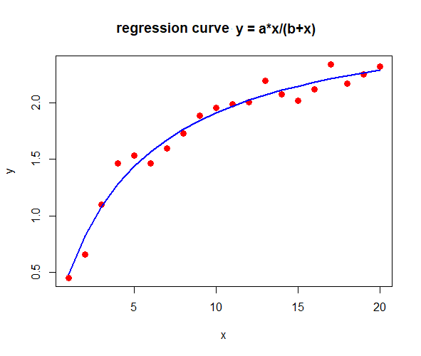
The R script above leads in the console the following output (up to randomisation) and produces the diagram below of data and regression curve.
Formula: y ~ a * x/(b + x)

Parameters:
  Estimate Std. Error t value Pr(>|t|)
a  2.84716    0.09288  30.653  < 2e-16 ***
b  4.91400    0.49858   9.856 1.12e-08 ***
---
Signif. codes:  0 ‘***’ 0.001 ‘**’ 0.01 ‘*’ 0.05 ‘.’ 0.1 ‘ ’ 1

Residual standard error: 0.09155 on 18 degrees of freedom

Number of iterations to convergence: 4
Achieved convergence tolerance: 3.995e-06

a = 2.847156 ,  b = 4.913995
correlation coefficient = 0.9857897
Warning message: In nls(formula = y ~ a * x/(b + x)) :
  No starting values specified for some parameters.
Initializing ‘a’, ‘b’ to '1.'.
Consider specifying 'start' or using a selfStart model

We extend this example to demonstrate that when we rewrite the nonlinear model into a corresponding linear model, it does produce a regression curve. However, this curve is of lower quality when we use the correlation between measurement data and model data as a metric. The parameter values also deviate significantly.
# apply a transformation to linear regression
reciprocal.x <- 1/x
reciprocal.y <- 1/y
# carry out linear regression
linfit <- lm(formula = reciprocal.y ~ reciprocal.x)
coeff <- coefficients(linfit)
# compute parameter values of nonlinear fit
alpha <- 1/coeff[1]
beta <- coeff[2]/coeff[1]
# compute modelling data
newfit <- alpha*x/(beta+x)
# display parameter values in console window and
# correlation between data and nonlinear fit obtained
# via transformation of given datas
cat("a =", alpha, ",  b=", beta, "\n")
cat("correlation coëfficient = ", cor(y,newfit), "\n")
# visualise data and regression curve
plot(x, y, type = "p", pch = 16, col = "red", cex = 1.3,
     main="regression curve y = a*x/(b+x) via transformation")
lines(x, newfit, type="l", col="blue", lwd=2)
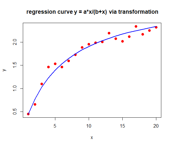
The above R script produces the following outputi n the console window and produces the below diagram of measurement data and regression curve.
a = 3.011385 ,  b= 5.805604
correlation coefficient =  0.9844066

The second regression curve is at first glance similar to the first one, but on closer inspection they differ from each other and the quality of the iterative nonlinear regression method is better.
What we can learn from this is that transformations from a nonlinear model to a linear model are rather dangerous when it comes to the quality of the model results, but they can provide suitable starting values for a nonlinear regression method
 Nonlinear regression

