Bi-exponential model of the head of a beer Every beer drinker is familiar with the phenomenon: when beer is poured into a glass, a head of the beer forms that disappears after a while if the glass remains untouched. The decreasing height of the head of a beer can be mathematically modelled reasonably well with a bi-exponential model. This approximation can be determined as follows (data file in csv format). The R script is executed and explained below in steps.

Step 1: reading in and plotting measured data

# read data from the csv file (measurements every 2 seconds)
data <- read.csv("beerfoam.csv", header = TRUE,
                     sep = ";", dec = ".", na.strings="", fill = TRUE)
t <- data$time    # time in sec
H <- data$height  # height of foam in cm
# plot measured data in a scatter plot
plot(t, H, type="p", pch=1, cex=0.7, col="red",
     xlab="t (in sec)", ylab="height (in cm)", 
     main="Height of foam versus time")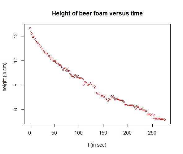

Step 2: describing the second part of measured data with exponential regression

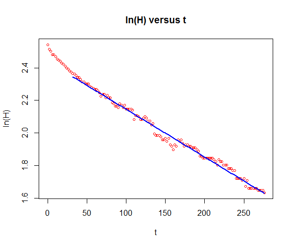
If you find an exponential growth model plausible, you can verify it by plotting the logarithm of the quantity against time as this should yield a straight line. In this specific case you see that over time, say when \(t>30\), a straight line does indeed describe the logarithm of the height well. You can then apply the exponential growth model to this selected piece.

The R script below produces the non-linear function fit and a matching diagram.

# plot ln(H.data) against t.data
plot(t, log(H), type="p", pch=1, cex=0.7, col="red",
     xlab="t", ylab="ln(H)", 
     main="ln(H) versus t")
# select data after 30 seconds
dataselection <- c(t.data>30)
ts <- t[dataselection]
Hs <- H[dataselection]
lnHs <- log(Hs)
# linear regression of ln(Hs) as linear function of t
fit <- lm(formula = lnHs ~ ts)
lines(ts, predict(fit), type="l", col="blue", lwd=2)

Next, we plot the measured data and the exponential growth model.

# plot measured data in a scatter plot and add the expontial fit
coeffs <- coefficients(fit)
a1 <- exp(coeffs[1])
r1 <- coeffs[2]
H_fit <- a1*exp(r1*t)
plot(t, H, type="p", pch=1, cex=0.7, col="red",
     xlab="t (in sec)", ylab="height (in cm)", 
     main="Height versus time with exponential model")
lines(t, H_fit, type="l", col="blue", lwd=2)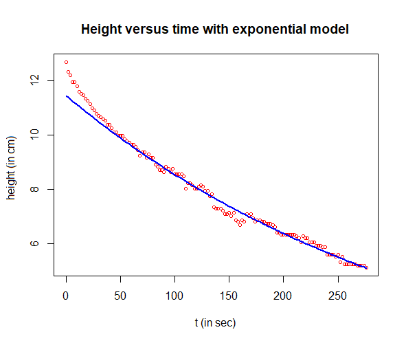

Step 3: plotting the residuals

The regression curve initially does not accurately describe the measurement data, but that is not the most important aspect. What matters is that the residuals once again exhibit an exponential decay pattern. The R script below illustrates this.

# compute residuals residuen and plot them
residuals <- H - H_fit
plot(t, residuals, type="p", pch=16, cex=0.7, col="red",
     xlab="t (in sec)", ylab="residual (in cm)", 
     main="residuals versus time")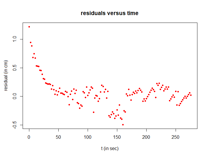

Step 4: describing the first part of measured data with exponential regression

We can calculate an exponential model for the first part of the residuals in the same way as before. For a change, let's perform a nonlinear fit with an estimate of initial parameter values using the method of partial sums. The R script below provides the exponential function fit of the residuals and a corresponding plot..

# select measured data in the first 60 seconds
dataselection <- c(t<60)
ts <- t[dataselection]
Rs <- residuals[dataselection]
# do a parameter estimation via partial sums
# by the way, logarithmic transformation works as well
N <- length(ts)/2
Nplus1 <- N+1
dt <- 2
s1 <- sum(Rs[1:N])
s2 <- sum(Rs[Nplus1:30])
r <- (log(s2)-log(s1)) / (N*dt)
h <- exp(r*dt)
a <- s1 * (1-h) / (1-h^N)
# apply nonlinear regression
nlfit <- nls(formula = Rs ~ a_2*exp(r_2*ts), start = list(a_2=a, r_2=r)) 
coeffs <- coefficients(nlfit) 
a2 <- coeff[1] 
r2 <- coeff[2] 
R_fit <- a2*exp(r2*t) # teken residuen in een scatterplot en voeg expontiële fit toe
plot(t, residuals, type="p", pch=16, cex=0.7, col="red",
     xlab="t (in sec)", ylab="residual (in cm)", 
     main="residuals versus time with exponential model")
lines(t, R_fit, type="l", col="blue", lwd=2)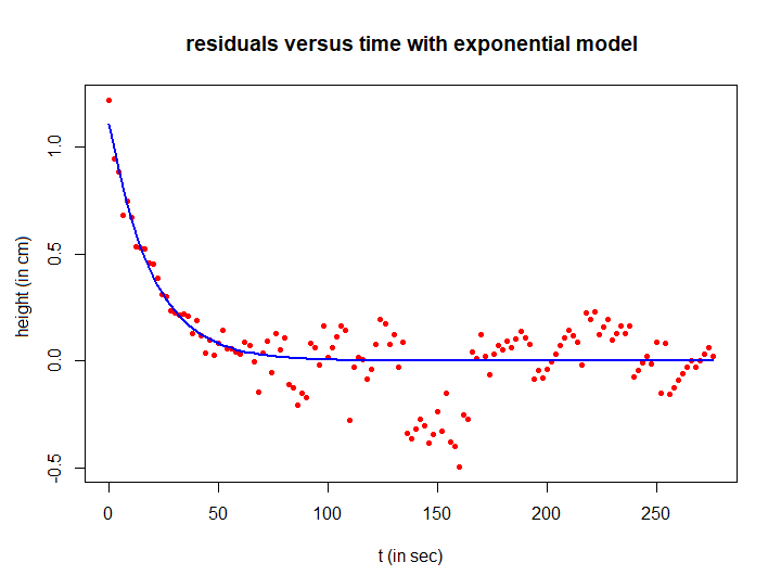 

Step 5: Putting all together

If we add both calculated regression curves, we obtain a nonlinear regression of the measured height of the beer foam over time:

# final result
plot(t, H, type="p", pch=1, cex=0.7, col="red",
     xlab="t (in sec)", ylab="height (in cm)", 
     main="Height of beer foam versus time plus bi-exponential model")
lines(t, H_fit + R_fit, type="l", col="blue", lwd=2)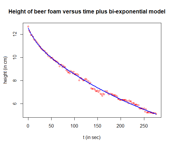

Step 6: Nonlinear regression with the final model and parameter estimates already found

It is even better to use the found parameter values as starting values for the following regression model \[\text{hoogte} = a_1\cdot e^{r_1\cdot t}+ a_2\cdot e^{r_1\cdot t}\] The R script below does the job.

# final nonlinear regression:
# apply bi-exponential regression 
nlfit <- nls(formula = H ~ a_1*exp(r_1*t) + a_2*exp(r_2*t),
             start = list(a_1=a1, r_1=r1, a_2=a2, r_2=r2))
print(summary(nlfit))  # print results
# plot the mmeasured data and the regression curve
plot(t, H, type="p", pch=1, cex=0.7, col="red",
     xlab="t (in sec)", ylab="height (in cm)", 
     main="Height of beer foam versus time plus bi-exponential model")
lines(t, predict(nlfit), type="l", col="blue", lwd=2)
# compute the correlation between measured data and modelling result 
cat("correlation coefficient =", cor(H,predict(nlfit)))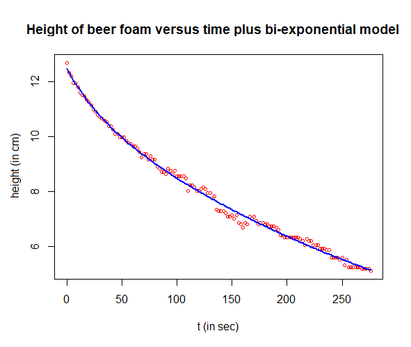

The final parameter estimates are tabulated below. The correlation coefficient between the measurement data and model results has also been calculated and printed. The end result is of high quality!

Formula: H ~ a_1 * exp(r_1 * t) + a_2 * exp(r_2 * t)

Parameters:
      Estimate Std. Error t value Pr(>|t|)    
a_1  1.121e+01  1.119e-01 100.191  < 2e-16 ***
r_1 -2.822e-03  5.164e-05 -54.641  < 2e-16 ***
a_2  1.284e+00  1.087e-01  11.815  < 2e-16 ***
r_2 -3.338e-02  5.665e-03  -5.892 2.89e-08 ***
---
Signif. codes:  0 ‘***’ 0.001 ‘**’ 0.01 ‘*’ 0.05 ‘.’ 0.1 ‘ ’ 1

Residual standard error: 0.1399 on 135 degrees of freedom

Number of iterations to convergence: 8 
Achieved convergence tolerance: 7.89e-06

correlation coefficient = 0.9975641

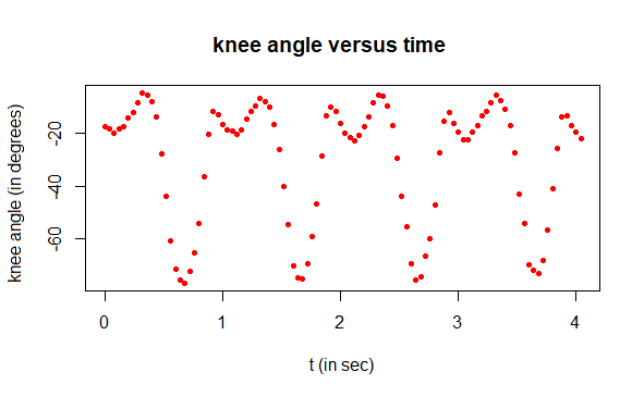
Knee angle during walking: harmonic analysis A girl's knee angle was measured while walking at a constant speed on a treadmill. The claim is that this angle can be describedwell as the sum of two sinusoids. This is an example of harmonic analysis. This approximation can be determined as follows. The R script is executed in steps.

Step 1: reading in and plotting measured data

# read data from csv file
kneedata <- read.csv("kneeanglemeasurement.csv", 
  header = TRUE, sep = ";", dec = ".", na.strings="", 
  fill = TRUE)
t <- kneedata$time    # time in sec
angle <- kneedata$angle  # knee angle in degrees
# plot knee angle data in a scatter plot
plot(t, angle, type="p", pch=16, cex=0.7, col="red",
     xlab="t (in sec)", ylab="knee angle (in degrees)", 
     main="knee angle versus time")

Step 2: describing measured data with sinusoidal regression

This resembles a periodic motion with a frequency of about 1 s^-1 . Let's first approach the measured data with a simple sinusoidal regression model \[\text{angle} = a_1\sin(b_1t+c_1)+d_1\] where the sine function takes arguments in degrees. For this we need to define a sine function in degrees in R. We estimate the starting values of the parameters for a nonlinear regression method as follows:

• from the frequency follows an estimate for the starting value of \(b_1\), namely: \(b_1=360\);
• we get the amplitude \(a_1\) as half the difference between extreme angular values;
• we estimate the vertical shift \(d_1\) of the sinusoid as the mean angular value because the time interval appears to be four periods;
• we initially estimate the phase angle to be equal to 0, for lack of a better answer.

The R script below produces the non-linear function fit and a matching diagram.

# define sine function in degrees instead of radians as input
sin_in_degrees <- function(degrees) {
  radians <- degrees*(pi/180)
  return(sin(radians))
}
# apply sinusoidal regression (with actually two components) 
fit1 <- nls( formula = angle ~ a1*sin_in_degrees(b1*t+c1) + d1, 
            start=list(a1=(max(angle)-min(angle))/2, 
                       b1=360, c1 = 0, d1=mean(angle)))
coeffs1 <- coefficients(fit1)
a1 <- coeffs1[1]
b1 <- coeffs1[2]
c1 <- coeffs1[3]
d1 <- coeffs1[4]
cat("a1 =", round(a1,2), "b2 =", round(b1,2), 
    "c1 =", round(c1,2), "d1 =", round(d1,2), "\n")
angle1 <- a1*sin_in_degrees(b1*t+c1) + d1
# plot measured data and regression curve
plot(t, angle, type="p", pch=16, cex=0.7, col="red",
     xlab="t (in sec)", ylab="knee angle (in degrees)", 
     main="knee angle versus time plus sinusoid")
lines(t, angle1, type="l", col="blue", lwd=2)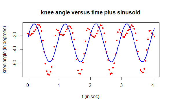

Step 3: plotting of residuals

The regression curve does not describe the measured data accurately, but that is not so important. What matters is that the residuals exhibit a periodic character once again. The R script below demonstrates this.

# compute residuals and plot them
residuals <- angle - angle1
plot(t, residuals, type="p", pch=16, cex=0.7, col="red",
     xlab="t (in sec)", ylab="residual (in degrees)", 
     main="residuals versus time")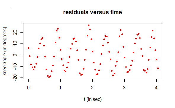

Step 4: describing of residuals with again sinusoidal regression

This appears to be a periodic motion with a frequency of approximately 2 s^-1. First, we'll approximate the residuals with a sinusoidal regression model \[\text{hoek} = a_2\sin(b_2t+c_2)+d_2\] where the sine function takes arguments in degrees. We estimate the initial values of the parameters for a nonlinear regression method in the following way:

• from the frequency, we obtain an estimate for the initial value of \(b_2\), namely: \(b_1=720\);
• the amplitude \(a_2\) is obtained as half of the difference between the extreme values of residuals;
• the vertical shift \(d_1\) of the sinusoid is estimated as close to 0. So we take \(d_2=0\);
• Looking at the graph, it appears to be the negative of a sine. This observation leads us to estimate \(c_2=180\) (corresponding with \(\pi\)).

The R script below gives the nonlinear function fit of the residuals and a corresponding diagram.

# apply sinusoidal regression (with actually two components) 
fit2 <- nls( formula = residuals ~ a2*sin_in_degrees(b2*t+c2) + d2, 
             start = list(a2=(max(residuals)-min(residuals))/2, 
                          b2=720, c2=180, d2=0))
coeffs2 <- coefficients(fit2)
a2 <- coeffs2[1]
b2 <- coeffs2[2]
c2 <- coeffs2[3] 
d2 <- coeffs2[4] 
cat("a2 =", round(a2,2), "b2 =", round(b2,2), 
    "c2 =", round(c2,2), "d2 =", round(d2,2), "\n")
angle2 <- a2*sin_in_degrees(b2*t+c2) + d2
# plot residuals and regression curve
plot(t, residuals, type="p", pch=16, cex=0.7, col="red",
     xlab="t (in sec)", ylab="residual (in degrees)", 
     main="residuals versus time plus sinusoid")
lines(t, angle2, type="l", col="blue", lwd=2)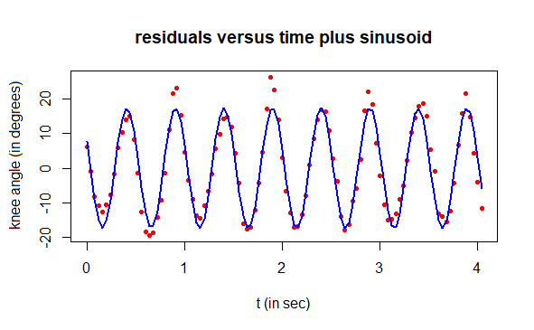

Step 5: putting it all together

If we add the two calculated regression curves, we have a nonlinear regression of the measured knee angles during walking:

# final result
plot(t, angle, type="p", pch=16, cex=0.7, col="red", ylim=c(-80,0),
     xlab="t (in sec)", ylab="knee angle (in degrees)", 
     main="knee angle versus time plus regression curve")
lines(t, angle1 + angle2, type="l", col="blue", lwd=2)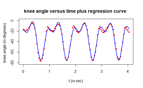

Step 6: Nonlinear regression with final model and parameter estimates already found

It is even better to use the parameter values found so for as starting values for the next regression model \[\text{height} = a_1\sin(b_1t+c_1)+a_2\sin(b_2t+c_2)+d\] The R script below does the job.

# ultimate nonlinear regression:
# apply sinusoidal regressie with twee sine functions 
nlfit <- nls(formula = angle ~ 
               a_1*sin_in_degrees(b_1*t+c_1) + 
               a_2*sin_in_degrees(b_2*t+c_2) + 
               d,
             start = list(a_1=a1, b_1=b1, c_1=c1, 
                          a_2=a2, b_2=b2, c_2=c2, 
                          d=d1))
print(summary(nlfit))  # print results
# plot the measured data and the regression curve
plot(t, angle, type="p", pch=16, cex=0.7, col="red", ylim=c(-80,0),
     xlab="t (in sec)", ylab="knee angle (in degrees)", 
     main="knee angle versus time plus regression curve")
lines(t, predict(nlfit), type="l", col="blue", lwd=2)
# compute the correlation between data and modelling results
cat("correlation coefficient =", cor(angle,predict(nlfit)))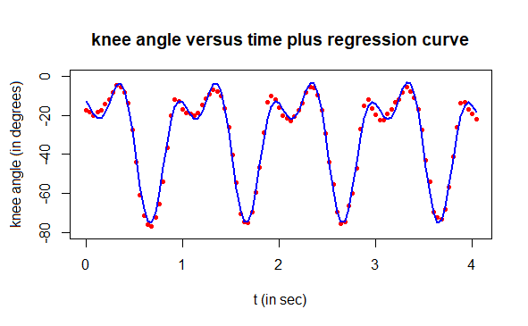

The final parameter estimates are tabulated below. Additionally, the correlation coefficient between measurement data and modelling results has been calculated and printed. The end result is of high quality!

Formula: angle ~ a_1 * sin_in_degrees(b_1 * t + c_1) + a_2 * sin_in_degrees(b_2 * t + c_2) + d

Parameters:
    Estimate Std. Error t value Pr(>|t|)    
a_1  27.2705     0.4548   59.96   <2e-16 ***
b_1 361.0197     0.8135  443.76   <2e-16 ***
c_1  23.1223     1.9446   11.89   <2e-16 ***
a_2  17.7445     0.4588   38.68   <2e-16 ***
b_2 723.3587     1.2204  592.72   <2e-16 ***
c_2 155.6522     2.8692   54.25   <2e-16 ***
d   -30.7267     0.3206  -95.83   <2e-16 ***
---
Signif. codes:  0 ‘***’ 0.001 ‘**’ 0.01 ‘*’ 0.05 ‘.’ 0.1 ‘ ’ 1

Residual standard error: 3.22 on 95 degrees of freedom

Number of iterations to convergence: 4 
Achieved convergence tolerance: 5.11e-06

correlation coefficient = 0.9908715