The logistic growth model Let's look at the initial value problem \[\frac{\dd y}{\dd t}=r\cdot y\cdot (1-y/K), \quad y(0)=y_0\] We specify the initial value problem in the form of an R function with the following three arguments:

• the independent variable, where we usually choose time \(t\);
• the initial state of the dependent variable, in this case the quantity \(y\);
• parameters, which here are the parameters \(r\) and \(K\).

The function returns a list of derivatives, but in this case it is just \(\frac{dy}{dt}\), and is used in the numerical method to solve the differential equation. In the code snippet below, the statement with(as.list(c(initialstate, parameters)). ...) ensures that the names of the parameters are available in the definition of the differential equation.

model <- function(time, initialstate, parameters){
  with(as.list(c(initialstate, parameters)), {
    dydt <-  r*y*(1-y/K)
    return(list(dydt))
  })
}

As initial value, parameter values, and the time interval, we successively choose:

y0 <- c(y=0.05)    # inital value of population density 
params <- c(r=0.1, # relative growth rate r
            K=10)  # carrying capacity K
t <- seq(from=0, to=100, by=0.5)  # time interval

The growth model is now solved with the ode instruction:

solution <- ode(y0, t, model, params)

The output is an object containing an array that tabulates the values of the dependent variable at specified times. You can use this to draw a graph of the solution curve. If you want to know more about how the initial value problem is solved numerically, use the diagnostics(solution) instruction.

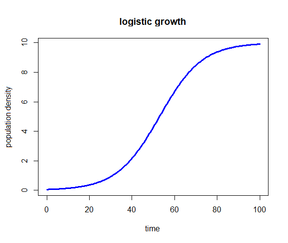
plot(solution, col="blue", main="logistic growth", 
     xlab="time", ylab="population density", lwd=3)

produces the following diagram: