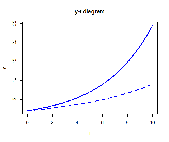
Two solution curves in one diagram We consider the exponential growth model \[\frac{\dd y}{\dd t}=r\cdot y\] at two different relative growth rates \(r\). The R script below

library("deSolve")

model <- function(time, initialstate, parameters) {
  with(as.list(c(initialstate, parameters)), {
    dydt <- r*y
    return(list(dydt))
  })
}

params1 <- c(r = 0.25)    # relative growth rate
params2 <- c(r = 0.15)    # idem
y <- c(y=2)               # initial value
t <- seq(0, 10, by = 0.1) # time interval

solution1 <- ode(y, t, model, params1)
solution2 <- ode(y, t, model, params2)

plot(solution1, solution2,
     main = "y-t diagram", xlab = "t", ylab="y", 
     lwd = 3, col = "blue"
)

yields the figure below.

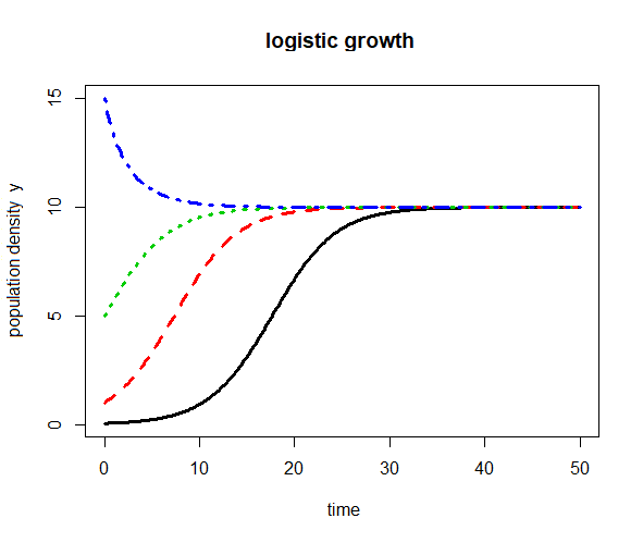
Multiple solution curves in one diagram Let us look at the logistic growth model \[\frac{dy}{dt}=r\cdot y\cdot(1-y/K)\] for multiple initial values \(y_0\). The R script below

library(deSolve)

model <- function(tijd, initialstate, parameters) {
  with(as.list(c(initialstate, parameters)), {
    dydt <- r*y*(1-y/K)
    return(list(dydt))
  })
}

y0 <- c(y = 0.05) # population density at the beginning
params  <- c(r = 0.3, # relative growth rate
             K = 10)  # carrying capacity
t <- seq(from = 0, to = 50, by = 0.1) # time interval


solution <- ode(y0, t, model, params)

# more initial values
y0s <- cbind(y = c(1, 5, 15))  
solutions <- list()
for (i in 1:nrow(y0s)) {
  solutions[[i]] <- ode(y0s[i,], t, model, params)
}

plot(solution, solutions, 
     main = "logistic growth", 
     xlab = "time", ylab="population density y", 
     lwd = 3)

yields the figure below.