System of linear GDVs Consider the following system of differential equations \[\left\{\begin{aligned} \frac{\dd x}{\dd t} &= a\cdot x+b\cdot y \\[0.25cm] \frac{\dd y}{\dd t} &=c\cdot x+d\cdot y\end{aligned} \right.\] with \[a=2,\quad b=-4,\quad c=2,\quad d=-3\] and initial values \[x(0)=2,\quad y(0)=3\]

The R script below

library(deSolve)

model <- function(time, initialstate, parameters) {
  with(as.list(c(initialstate, parameters)), {
    dxdt <- a*x + b*y
    dydt <- c*x + d*y
    return(list(c(dxdt, dydt)))
  })
}

params  <- c(a = 2, b = -4, c = 2, d = -3) # parameters       
xy0 <- c(x = 2, y = 3)    # initial values
t <- seq(0, 10, by = 0.1) # time interval

solution <- ode(xy0, t, model, params)

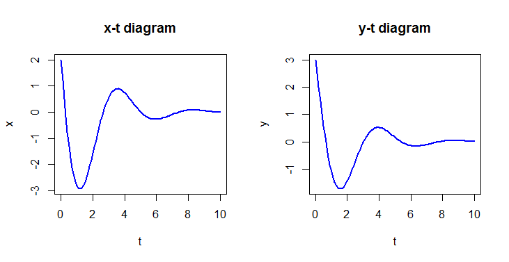
plot(solution, main = c("x-t diagram", "y-t diagram"),
     xlab = "t", ylab = c("x", "y"), lwd = 2, col = "blue")

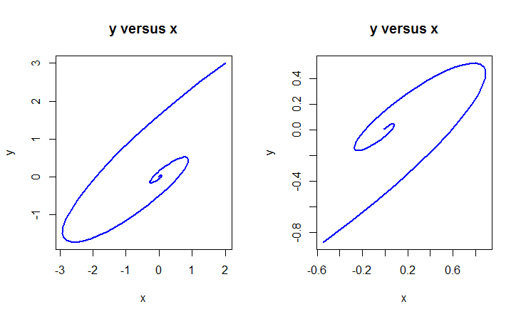
plot(solution[, "x"], solution[, "y"], type = "l", 
     main = "y versus x", xlab = "x", ylab = "y", 
     lwd = 2, col = "blue")

xy <- subset(solution, select = c("x", "y"), 
             subset = -1<x & x<1 & -1<y & y<1)
plot(xy, type = "l", main = "y versus x", 
     xlab = "x", ylab = "y", lwd=2, col = "blue")

yields the following diagrams