Doing mathematics with R: Differential equations in R
 Parameter estimation in differential equations
We have already seen how parameter values can be optimised through regression analysis for explicit solutions of differential equations. The FME package with its dependent R packages also allows the user to fit parameters in differential equations to measured data. We give an example of quantitative pharmacokinetics, namely that of oral administration of a drug which is subsequently eliminated from the human body.
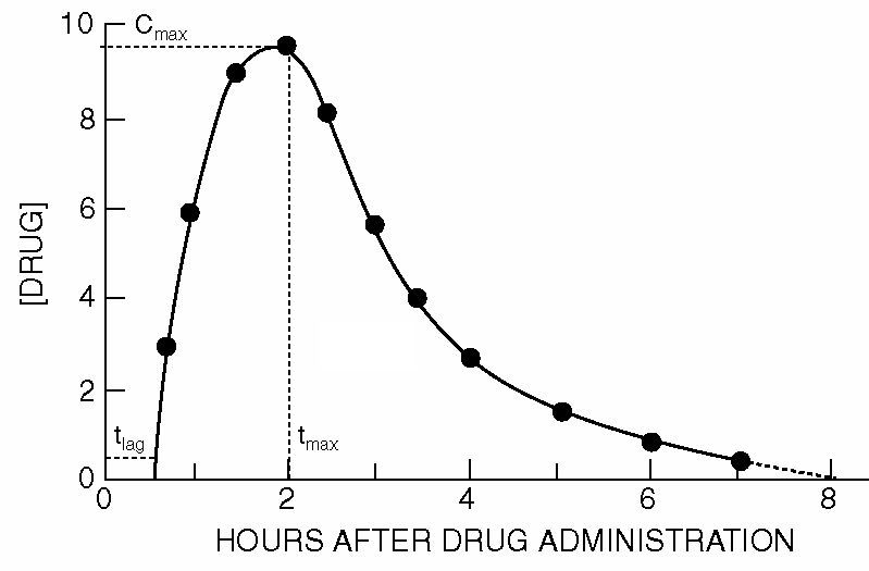
Oral administration of a drug with first-order kinetics of absorption and elimination Propranolol is a beta-blocker that is used, among other things, to lower blood pressure. When administered orally, i.e. swallowing tablets or consuming medicated drink, the drug enters the stomach first. With some delay, the drug then enters the small intestine; the delay can be seen in a concentration-time curve because the concentration does not start to rise until some time ( \(t_\text{lag}\) ) after oral administration. From the small intestine, the drug enters the liver through a diffusion process via the portal vein. The absorption process mainly follows first-order kinetics in this step due to passive diffusion. However, the liver allows only a limited portion to pass unchanged into the general blood circulation of the body (beyond the portal vein and the liver). The drug that has passed through the blood then spreads further over the body and can have its therapeutic effect. The fraction of the administered drug that enters the general blood circulation unchanged is referred to as the bioavailability of the drug in the Dutch literature.
As soon as the absorbed drug is distributed throughout the body (this can also take place in different tissues and body fluids), it also undergoes the process of elimination. Initially, the amount absorbed exceeds the amount eliminated, resulting in an increase in plasma concentration. At the maximum, the absorption is equal to the elimination. Over time, as the absorption process comes to an end, elimination predominates; the concentration then decreases over time. The graph below shows the typical shape of the concentration-time curve for an orally administered drug.

The above curves belong to a bi-exponential model, but we can also describe it in another way, namely as a dynamical system. The diagram below shows a graphical representation of the model for oral administration of a drug with first-order kinetics for absorption in and elimination from the body, considered as one central compartment:

This picture represents the following: the drug is absorbed from the small intestine and partly ends up in the general blood circulation via the liver. For the removal of the drug from the small intestine we use an exponential model with elimination rate constant \(k_a\). So: \[\frac{\dd A_\text{small intestine}}{\dd t} = -k_a\cdot A_\text{small intestine}\] where \(A_\text{small intestine}\) is the amount of the orally administered drug in the small intestine. The rate at which it enters the general circulation is of opposite sign and only a fraction of the drug passes through the small intestine and liver. We account for this in the corresponding increase in the plasma concentration \(C\) of the drug with an efficacy constant \(\mathrm{eff}\), which depends on the bioavailability and the volume of distribution. Together with the first-order kinetics of elimination from the body, we can write in mathematical language: \[\frac{\dd C}{\dd t} = k_a\cdot \mathtt{eff}\cdot A_\text{small intestine} -k_e\cdot C\] So we have a system of differential equations.
We fit the three parameters \(k_a\), \(k_e\) and \(\mathtt{eff}\) using literature data from the following article
Olanoff, L. S., Walle, T., Cowart, T. D., Oexmann, M. J. & Conradi, E. C. (1986). Food effects on propranolol systemic and oral clearance: support for a blood flow hypothesis. Clinical Pharmacology and Therapeutics , 40 , 408-414.
Implementation and parameter estimation in R For convenience we denote the amount of propranolol in the small intestine with \(x\) and the plasma concentration with \(y\). We then have the following system of differential equations: \[\left\{\begin{aligned} \frac{\dd x}{\dd t} &=-k_a\cdot x \\ \\ \frac{\dd y}{\dd t} &= k_a\cdot \mathtt{eff}\cdot x -k_e\cdot y\end{aligned}\right.\] For parameter estimation, we use the Flexible Modeling Environment ( FME) package and its dependent packages deSolve, rootSolve, and coda. An alternative is the grind ( GReat INtegrator Differential equations) package as a user interface to the underlying R packages, but we will not exemplify this.
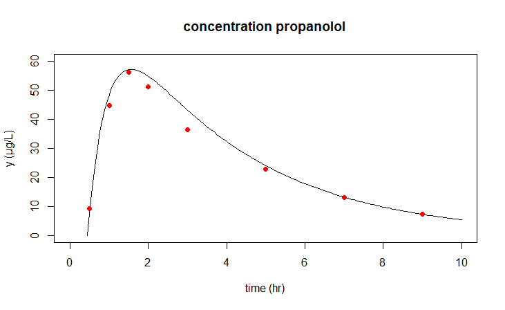
The R script below uses the ode instruction from the deSolve package to numerically calculate the solution curve for estimated parameter values. In the plot instriction from the package we plot the measured data together with the solution curve in one daigram.
library("FME")

model <- function(time, initialstate, parameters) {
  with(as.list(c(initialstate, parameters)), {
    dxdt <- -ka*x
    dydt <- ka*x*eff - ke*y
    list(c(dxdt, dydt))
  })
}

data <- data.frame(
  time = c(0.5, 1, 1.5, 2, 3, 5, 7, 9),
  y = c(9.15, 44.82, 56.29, 51.33, 36.43,
         22.89, 13.06, 7.21)
)

params <- c(ka = 2, ke = 0.3, eff = 1)
xy0 <- c(x = 80, y = 0)
t <- seq(from = 0.45, to = 10, by = 0.05)

solution <- ode(xy0, t, model, params)

plot(solution, obs = data,
     xlim = c(0,10), ylim = c(0,60),
     main = "concentration propanolol",
     xlab = "time (hr)", ylab = "y (µg/L)",
     obspar = list(pch=16, col="red"))
We have estimated reasonable parameter values based on literature data, but we can also use these values as starting values for a systematic improvement of the model results in relation to the measurement data.
To do this end, define a cost function using modCost to estimate the residual deviation between model results and measurement data.
cost <- function(p) {
  opl <- ode(xy0, t, model, p)
  dimnames(opl) <- list(NULL, c("time", "x", "y"))
  modCost(opl, data, x="time", weight = "none")
}
After this we can try to achieve better parameter values with the modFit command at certain starting values. Code snippet below
params <- c(ka = 2, ke = 0.3, eff = 1)
modelfit <- modFit(f = cost, p = params)
print(summary(modelfit))
leads to a display of better parameter values in the console window:
Parameters:
    Estimate Std. Error t value Pr(>|t|)
ka   2.25216    0.31238    7.21 0.000800 ***
ke   0.29163    0.02684   10.87 0.000115 ***
eff  0.90873    0.04931   18.43 8.65e-06 ***
---
Signif. codes:  0 ‘***’ 0.001 ‘**’ 0.01 ‘*’ 0.05 ‘.’ 0.1 ‘ ’ 1

Residual standard error: 2.206 on 5 degrees of freedom
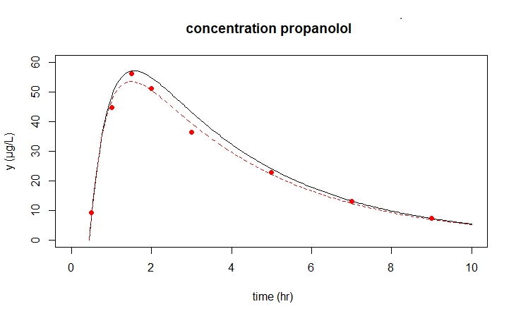
Finally, in one figure we show the previously calculated model outcomes and the improved outcomes for \(k_a=2.252\), \(k_e = 0.292\) and \(\text{eff}=0.909\).
sol1 <- ode(xy0, t, model, params)
sol2 <- ode(xy0, t, model, coef(modelfit))
plot(opl1, pl2, obs = data,
     xlim = c(0,10), ylim = c(0,60),
     main = "concentration propanolol",
     xlab = "time (hr)", ylab = "y (µg/L)",
     obspar = list(pch=16, col="red")
)


