In a pharmacokinetic model with a prescription for medication dosage or in control systems, there are events that change the equations. With repeated intravenous injections, there are moments when the concentration of a drug sharply increases. In a physics example of a bouncing ball, at the collision of the falling ball with a horizontal surface, the direction and speed of the ball will change abruptly. A biomedical example of the latter type of events is a control system, where events affect the behaviour of a system, such as maintaining blood sugar levels in the human body. You can also create such models using the deSolve package. We illustrate this using a onr-compartment model of repeated intravenous injections, but this is also applicable to a 2-compartment model of repeated oral administration of medication. We also consider an example of population management by capture (or harvesting, depending on the context), where once a population reaches a certain size by capture, it is abruptly reduced by capture.
We consider a one-compartment model with first-order kinetics for elimination of the antibiotic Ceftazidime and a series of equal-dose bolus injections administered at regular intervals. Henceforth, we denote the dosing interval as \(\tau\). Realistic pharmacokinetic parameter values are a repeated dosage \(D=1000\,\text{mg}\), an elimination constant \(k = 0.034\,\text{h}^{-1}\), and a volume of distribution \(V_d=20.6\,\text{L}\), which allow you to calculate the \(C\) plasma concentration of the drug from the amount \(A\) of the drug in the bloodstream using the formula \(C =A / V_d\). These data come from a scientific study of patients suffering from chronic renal insufficiency (M.A.Demotes-Mainard, F., Vincon, G., Ragnaud, J.M., Morlat, P., Bannwarth, B. & Dangoumau, J. (1993). Journal of Clinical Pharmacology, 33, 475-479). Pharmacokinetic parameters values for drug can also be found in Dutch information texts registered by the 'Medicine Evaluation Board'; see, for example, the websites www.cbg-meb.nl and www.geneesmiddelenrepertorium.nl .
We give two implementations in R, where the second method via events is highly preferred because it does not depend on the numerical method for solving the differential equation and is actually the easiest.
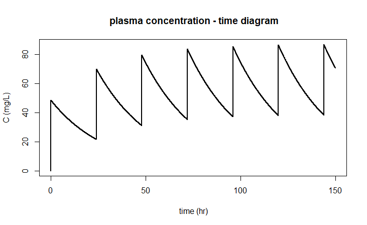
In this pharmacokinetic model, between injections we have the ODE \[\frac{\dd C}{\dd t}=-k\cdot C\] and after each administration interval \(\tau\) when another bolus injection occurs, the plasma concentration rises abruptly with \(D/V_d\). The computer model cannot raise the concentration abruptly, but we can set it up in such a way that after each injection in a short time, say in the time period \(\delta\), a linear increase in the plasma concentration leads to the desired increase. In other words, we adjust the function that yields the derivative for the solution method.
The following R script
library(deSolve)

delta <- 1/100

model <- function(time, initialstate, parameters) {
  with(as.list(c(initialstate, parameters)), {
    if (time %% tau <= delta) {
      u <- (D/Vd)/ delta
    } else {
      u <- 0
    }
    dCdt <- -k*C + u
    list(c(dCdt))
  })
}

params <- c( k = 0.034,  # elimination constant
             Vd = 20.6,  # volume of distribution
             D = 1000,   # dose
             tau = 24    # administration interval
             )
t <- seq(from = 0, to = 150, by = delta) # time interval
C0 <- c(C = 0) # initial values

solution <- ode(C0, t, model, params)

plot(solution, type = "l", lwd = 2,
     xlab = "time (hr)", ylab = "C (mg/L)",
     main = "plasma concentration - time diagram")
leads to the following diagram:

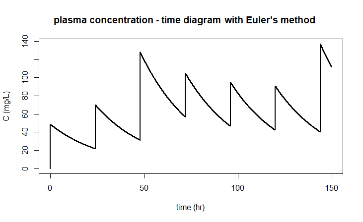
The above implementation does depend on the method in which the system is solved. If you were to apply the Euler method in the ode instruction (via method="euler" ), you would not get a good graph because, for example, after 48 hours the interval of drug administration is not properly recognised:

In this pharmacokinetic model, between injections we have the ODE \[\frac{\dd C}{\dd t}=-k\cdot C\] and after each administration interval \(\tau\) when another bolus injection occurs, the plasma concentration rises abruptly with \(D/V_d\). We do this now not through the derivative, but through the quantity itself. The injections are specified through a special event that take place at known times. In a dataframe you specify
- the name of the state variable that changes value;
- the times when the changes must take place;
- the strength of the change;
- the nature of the change (replace, add, multiply).
For the rest, you specify in the usual way how the model behaves between events and in the ode instruction you introduce the events option.
The following R script
library(deSolve)

model <- function(time, initialstate, parameters) {
  with(as.list(c(initialstate, parameters)), {
    dCdt <- -k*C
    list(c(dCdt))
  })
}

params <- c(k = 0.034)  # elimination constant

D <- 1000  # dose
Vd <- 20.6 # volume of distribution
tau <- 24  # administration interval

injection <- data.frame(var = "C",
                        time = seq(
                          from = 0,
                          to = 150,
                          by = tau),
                        value = D/Vd,
                        method = "add")

t <- seq(from = 0, to = 150, by = 1) # time interval
C0 <- c(C = 0) # initial values

solution <- ode(C0, t, model, params,
                 events = list(data = injections))

plot(solution, type = "l", lwd = 2,
     xlab = "time (hr)", ylab = "C (mg/L)",
     main = "plasma concentration - time diagram")
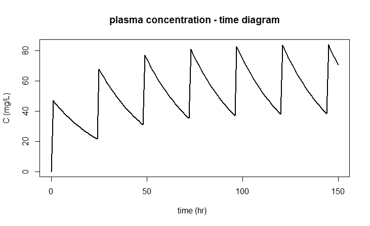
leads to the following diagram:

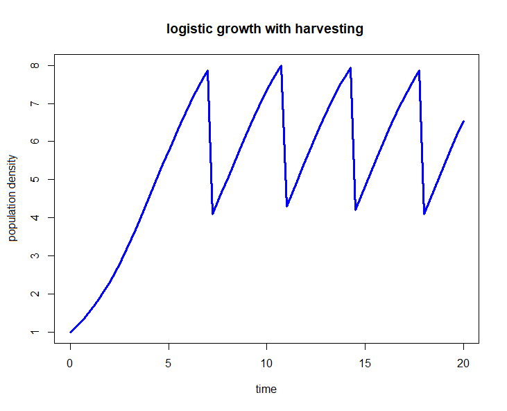
We consider a population model of logistic growth given by the following differential equation \[\frac{\dd y}{\dd t}=r\cdot y\cdot \left(1-\frac{y}{K}\right)\] for certain values of the relative growth rate constant \(r\) and the carrying capacity \(K\). But when the population density \(y\) has reached \(80\%\) of its maximum size, it is abruptly halved by harvesting, only to be left untouched again until this event occurs again. This form of event-based regulation can also be simulated in mathematical software.
For convenience we choose \(r=0.5\), \(K=10\) and \(y(0)=1\), but the implementation of the population model is formulated in general terms so that you can easily choose other values. The harvesting is triggered when a certain condition is met: in this case, when the population density \(y\) becomes equal to \(0.8K\). The triggering of the event is controlled in the deSolve package via rootfunc, a function that should signal that \(y-0.8K\) reaches the value \(0\). The handling of the event, that is, what has to happen when the event is triggered, is controlled in the eventfunc function: in this case we halve the population density. In the R script below you see how this can be done. The bottom line is that you have to give the name rootfunc and eventfunc as options in the ode command.
library(deSolve)

model <- function(time, initialstate, parameters){
  with(as.list(c(initialstate, parameters)), {
    dydt <-  r*y*(1-y/K)
    list(dydt)
  })
}

rootfunc <- function(t, y, parameters) {
  with(as.list(c(parameters)), {
    return(y-0.8*K)
  })
}

eventfunc <- function(t, y, parameters) {
  y <- y/2
  return(y)
}

y0 <- c(y=1)
params <- c(r=0.5, K=10)
t <- seq(from=0, to=20, by=0.25)

solution <- ode(y0, t, model, params,
                rootfun = rootfunc,
                events = list(func = eventfunc,
                              root = TRUE)
            )

plot(solution, col="blue", lwd = 3,
     main = "logistic growth with harvesting",
     xlab = "time", ylab="population density")
This R script above leads to the following diagram:

 Differential equations with events

