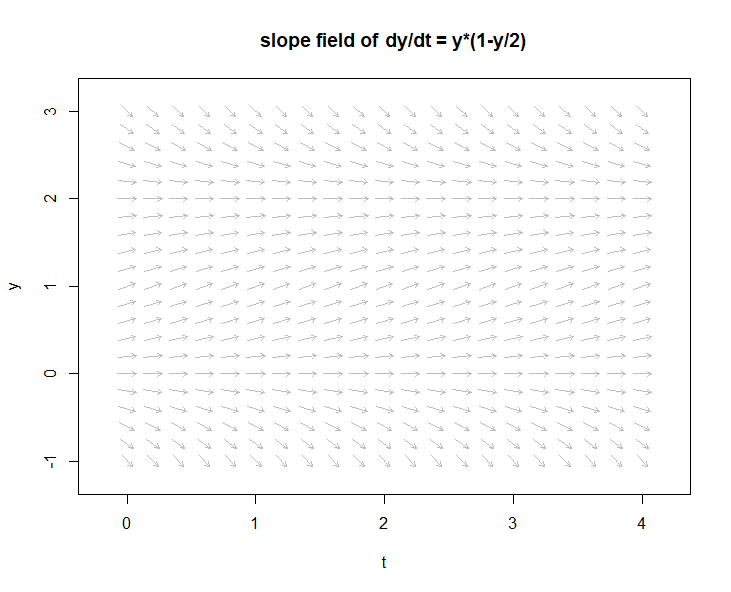
For an autonomous dynamical system of first order, i.e., a differential equation of the form \[\frac{\dd y}{\dd t}=\varphi(y)\] for some function \(\varphi\), a slope field can be plotted in R using the phaseR package. We use this package because it offers even more facilities (e.g., for phase plane analysis and for systems of two autonomous differential equations). We give two examples: a line element field without and one with some solution curves.
The R command for plotting a slope field is called flowField, because it is also used to plot a vector field for systems of two differential equations. We illustrate the use of the R instruction using the logistic differential equation \[\frac{\dd y}{\dd t}=y\cdot (1-y/2)\] The R script below
library(phaseR)

model <- function(time, initialstate, parameters){
  with(as.list(c(initialstate, parameters)), {
    dydt <-  r*y*(1-y/K)
    return(list(dydt))
  })
}

params <- c(r = 1, K = 2)

flowField(model, xlim = c(0, 4), ylim = c(-1, 3),
          parameters = params, system = "one.dim",
          state.names = c("y"), add = FALSE,
          xlab = "t", ylab = "y",
          main = "slope field of dy/dt = y*(1-y/2)")
leads to the following diagram:

With the add = FALSE option you indicate that you want to plot a new diagram and not add the slope field to an existing figure (via add = TRUE ). The option system = "one.dim" indicates that we are dealing here with an autonomous first-order differential equation and not with a system of two differential equations (then use system = "two.dim" ). We specify the dependent variable via state.names = c("y") because we did not use this variable name in the model function (we used initialstate as an argument instead)
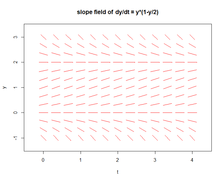
Instead of lineal elements, the flowField instruction draws arrows in the diagram. The code fragment below illustrates how you can simulate lineal segments by adjusting the size of the arrowhead and how you can specify the colour and granularity of the grid via options.
We refer to the phaseR manual for more details about the different options in the flowField function.
flowField(model, xlim = c(0, 4), ylim = c(-1, 3),
          parameters = params, system = "one.dim",
          state.names = c("y"), points = 13,
          arrow.head = 0.001, col = "red",
          add = FALSE, xlab = "t", ylab = "y",
          main = "slope field of dy/dt = y*(1-y/2)")

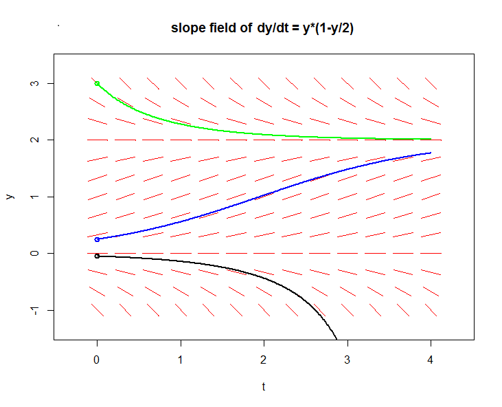
We can add solution curves To a slope field via the trajectory function. The R script below
flowField(model, xlim = c(0, 4), ylim = c(-1, 3),
          parameters = params, system = "one.dim",
          state.names = c("y"), points = 13,
          arrow.head = 0.001, col = "red",
          add = FALSE, xlab = "t", ylab = "y",
          main = "slope field of dy/dt = y*(1-y/2)")

trajectory(model, parameters = params, system = "one.dim",
           state.names = c("y"), y0 = c(0.25), tlim = c(0, 4),
           col = "blue", lwd = 2)
trajectory(model, parameters = params, system = "one.dim",
           state.names = c("y"), y0 = c(3), tlim = c(0, 4),
           col = "green", lwd = 2)
trajectory(model, parameters = params, system = "one.dim",
           state.names = c("y"), y0 = c(-0.05), tlim = c(0, 4),
           col = "black", lwd = 2)
leads to the following diagram, which is commonly called a phase portrait of an ODE:

We refer to the phaseR manual for more details about the different options in the flowField and trajectory functions.
 Slope field and phase portait of an autonomous first-order differential equation


