Basic skills in R: Working with data structures
 Table
Table
- What is a table in R?
- First R example of a frequency table: a book collection
- Second R example of a frequency table and bar chart: simulation of rolling dice
- R example of a two-way contingency table
- R example of a three-way contingency table
- List of functions for creating and manipulating tables in R
- Practice
What is a table in R? In R, the object created with the function table() is usually a frequency table or a contingency table summarising categorical data, i.e, named characteristics of individuals or objects that do not have magnitude on a numerical scale.
A frequency table, also called one-way table, consists of only two columns: one for the categorical variable and one for the absolute frequency of each category in a dataset. It can be graphically displayed in a bar chart (also known as bar graph or bar diagram) or summarised into a histogram. When the absolute frequencies are divided by the total number of objects in the dataset, the numbers indicate a proportion or relative frequency (or a percentage when we also multiply by 100) and then we get the relative frequency distribution, also referred to as the probability distribution of the categorical variable.
An example is a set of books which are categorised according to genre and for each category (we distinguish here three categories 'Fantasy', 'Science function', and 'Thriller') one counts the number of books that belong the category. Then, the (absolute) frequency table could look as follows:
| Book genre (categorical variable) |
Number of books in each genre (absolute frequency) |
| Fantasy | 11 |
| Science fiction | 15 |
| Thriller | 6 |
A contingency table (also called cross table or cross tabulation) is an absolute frequency table for two (or more) categorical variables. So, it gives the absolute frequencies of occurrence of all combinations of two (or more) categorical variables. In the example below we consider a group of people and use two categorical variables with two categories each: eye colour (blue or brown) and use of visual support tool (yes, 'wearing glasses' or no, 'not wearing glasses'). Then, the contingency table with absolute frequencies could look as follows:
| use of a visual support tool |
||
| eye colour | wearing glasses |
not wearing glasses |
| blue |
7 | 18 |
| brown | 12 | 34 |
Quite often, for data analysis purposes, total sums of rows and of columns are added; the sums are called the marginal totals. In our example the frequency table would look like
| use of visual support tool |
|||
| eye colour | wearing glasses |
not wearing glasses |
row sum |
| blue |
7 | 18 | 25 |
| brown | 12 | 34 | 46 |
| column sum |
19 | 52 | 71 |
By the way, the observed and expected value of eye colour and use of a visual support tool are in this example the same, as can be checked with the given marginal sums of the observed data
First R example of a frequency table: a book collection How to create a table in R, or more precisely how to create a frequency table? The basic idea is that you first create a vector in which you list for each object in your data set the corresponding category in the categorical variable you are interested in. Next you apply the function table() to the data vector to generate the frequency table.
We illustrate this by an example of an imaginary private book collection. Suppose that this collection consists of 9 book belonging to 4 genres: Thriller, Fantasy, Science fiction and Detective. So, the genre of the book is the categorical variable we are interested in. First, create a vector, say books in which the genre of each book of the collection is listed.
> books <- c("Thriller", "Thriller", "Fantasy", "Detective", "Detective",
+            "Thriller", "Fantasy", "Detective", "Science fiction")
To create the absolute frequency table of the given data set, let's call it abs_freq_table, you only have to apply the function table() to the vector that you just created. The R function does all the counting for you!
> abs_freq_table <- table(books)
> abs_freq_table
books
      Detective         Fantasy Science fiction        Thriller
              3               2               1               3
To create the relative frequency table, you could use basic calculus and enter the instruction abs.freq.table/length(books) or instead use the built-in function prop.table(); multiply by 100 to get the relative frequencies as percentages.
> abs_freq_table / length(books)
books
      Detective         Fantasy Science fiction        Thriller
      0.3333333       0.2222222       0.1111111       0.3333333
> prop.table(abs_freq_table)
books
      Detective         Fantasy Science fiction        Thriller
      0.3333333       0.2222222       0.1111111       0.3333333
> prop.table(abs_freq_table)*100
books
      Detective         Fantasy Science fiction        Thriller
       33.33333        22.22222        11.11111        33.33333
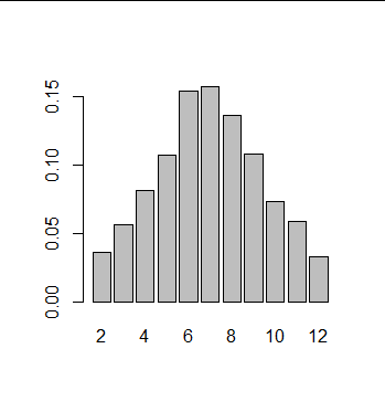
Second R example of a frequency table and bar chart: simulation of rolling dice In the second example we simulate the rolling of a fair die and make a frequency table in the same way as in the previous example for the categorical variable of possible outcomes. In addition we show how a bar chart can be created.
First we set the seed of our random number generator so that we get the same data generated whenever we repeat the sample session. We generate a random sequence of outcomes of throwing dice.
> set.seed(123)
> rolls <- sample(1:6, size=50, replace=TRUE)
The creation of the frequency table is done with the function table():
> abs_freq_table <- table(rolls)
> abs_freq_table
rolls
 1  2  3  4  5  6
 9  8 11  6  9  7
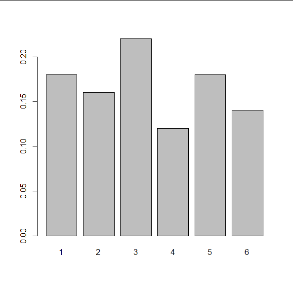
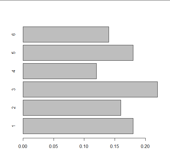
We turn it into a relative frequency table via the function prop.table() (short for proportion table):
> rel_freq_table <- prop.table(abs_freq_table)
> rel_freq_table
rolls
   1    2    3    4    5    6
0.18 0.16 0.22 0.12 0.18 0.14
We can visualise the relative frequency table as a bar chart by the function barplot() and the true/false option horiz determines whether we have vertical bars (default) or horizontal bars:
> barplot(rel_freq_table)
> barplot(rel_freq_table, horiz=TRUE)
Fancier bar charts can be created with the ggplot2 package in R.
R example of a two-way contingency table For two-way tables, the format for the function table() is crosstab <- table(A,B) where A is the row variable and B is the column variable, each of them being a vector. In our example, the categorical row variable is the sex (letter "M" for Male and "F" for Female) of persons in a particular group who we have asked what their favourite flavour of ice cream is (the categorical variable with letter type categories "C" for Chocolate, "S" for Straberry, and "V" for Vanilla).
Our sample session starts with entering the date in two vectors, followed by the creation of the two-way contingency table. We follow here the convention of placing the nominal data (male and female) in rows and ordinal data (the three flavours) in columns
> sex <- c("M", "F", "M", "M", "F", "F", "M", "F")
> preference <- c("C", "V", "V", "C", "C", "S", "S", "C")
> crosstab <- table(sex, preference)
> crosstab
   preference
sex C S V
  F 2 1 1
  M 2 1 1
To make the output more readable, you can change the individual row and column names via the function dimnames():
> dimnames(crosstab)[[1]] <- c("female", "male")
> dimnames(crosstab)[[2]] <- c("chocolate", "strawberry", "vanilla")
> crosstab
        preference
sex      chocolate strawberry vanilla
  female         2          1       1
  male           2          1       1
You can use the function addmargins() to add marginal totals to a contingency table.
> addmargins(crosstab)
        preference
sex      chocolate strawberry vanilla Sum
  female         2          1       1   4
  male           2          1       1   4
  Sum            4          2       2   8
Proportions can be computed via the function prop.table() with respect to rows (option margin=1) or columns (margin=2).
> prop.table(crosstab, margin=1)
        preference
sex      chocolate strawberry vanilla
  female      0.50       0.25    0.25
  male        0.50       0.25    0.25
> addmargins(prop.table(crosstab, margin=1), margin=2)
        preference
sex      chocolate strawberry vanilla  Sum
  female      0.50       0.25    0.25 1.00
  male        0.50       0.25    0.25 1.00
From the above contingency tables it is immediately clear that there exists in our made-up data set no difference in preference of flavour of ice cream between males and females.
> prop.table(crosstab, margin=2)
        preference
sex   chocolate strawberry vanilla
  female       0.5        0.5     0.5
  male         0.5        0.5     0.5
> addmargins(prop.table(crosstab, margin=2), margin=1)
        preference
sex      chocolate strawberry vanilla
  female       0.5        0.5     0.5
  male         0.5        0.5     0.5
  Sum          1.0        1.0     1.0
Without the directions,
prop.table() computes relative frequencies with respect to the size of the group of persons.
> addmargins(prop.table(crosstab))
        preference
sex      chocolate strawberry vanilla   Sum
  female     0.250      0.125   0.125 0.500
  male       0.250      0.125   0.125 0.500
  Sum        0.500      0.250   0.250 1.000
R example of a three-way contingency table As an example of a three-way contingency table we use the Arthritis dataset included with the vcd package. The data are from
Koch, G. and S. Edwards (1988). Clinical efficiency trials with categorical data. In: K. E. Peace (Ed.), Biopharmaceutical Statistics for Drug Development (pp. 403–451) New York: Marcel Dekker
Also in: Statistical Analysis with Missing Data (2nd ed., Eds. R. J. A. Little and D. Rubin) Hoboken, NJ: John Wiley & Sons, 2002.
It represents a double-blind clinical trial of new treatments for rheumatoid arthritis.
So in the R sample session we first install the vcd package with the function install.packages() and activate this package with the function library(); just ignore the feedback messages in the console window for the moment.
> install.packages("vcd")
> library(vcd)
The first few observation data can be seen via the function head():
> head(Arthritis)
  ID Treatment  Sex Age Improved
1 57   Treated Male  27     Some
2 46   Treated Male  29     None
3 77   Treated Male  30     None
4 17   Treated Male  32   Marked
5 36   Treated Male  46   Marked
6 23   Treated Male  58   Marked
The Arthitis object is a data frame, which is a data structure that we will discuss later, but it contains three categorical variables: Treatment (Placebo, Treated), Sex (Male, Female), and Improved (None, Some, Marked). Below we use the function with() so that we can use the names of the categorical variables without using long names referring constantly to the Arthritis object via long names such as Arthritis$Treatment. When we look at the three-way table that we create with table(), then we get for each sexual category a two-way table of the remaining categorical variables Treatment and Improved.
> three_way_table <- with(Arthritis, table(Treatment, Improved, Sex))
> three_way_table
, , Sex = Female
         Improved
Treatment None Some Marked
  Placebo   19    7      6
  Treated    6    5     16

, , Sex = Male

         Improved
Treatment None Some Marked
  Placebo   10    0      1
  Treated    7    2      5
Marginal totals can be added again via the function addmargins():
> addmargins(three_way_table, margin=c(1,2))
, , Sex = Female

         Improved
Treatment None Some Marked Sum
  Placebo   19    7      6  32
  Treated    6    5     16  27
  Sum       25   12     22  59

, , Sex = Male

         Improved
Treatment None Some Marked Sum
  Placebo   10    0      1  11
  Treated    7    2      5  14
  Sum       17    2      6  25
A more compact, flattened table can be made with the function ftable().
> ftable(three_way_table)
                   Sex Female Male
Treatment Improved
Placebo   None             19   10
          Some              7    0
          Marked            6    1
Treated   None              6    7
          Some              5    2
          Marked           16    5
List of functions for creating and manipulating tables in R
| Function | Description |
table(var1, var2, ..., varN) |
Create an N-way contingency table from N categorical variables; a 1-way contingency table is better known as a frequency table. |
prop.table(table, margin=...) |
Express table entries as fractions of marginal totals defined by the margin option. |
addmargins(table, margin=...) |
Put marginal totals defined by the margin option on a table. |
ftable(table) |
Create a compact, 'flat' contingency table from a given one. |
dimnames(table) |
Retrieve or set the dimensional names of the given table. |
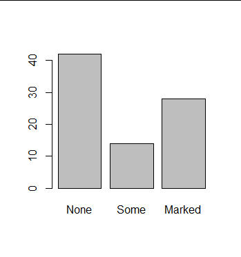
Practice 1. Arthritis example
We continue to work with the Arthritis data set of the vcd package and ask you to
- create a frequency table of the categorical variable
Improvedand plot a bar chart of this frequency table. - create a two-way table of the variables
TreatmentandImproved.
2. Randomly grabbing skittles
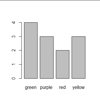
Imagine that you randomly grab a handful of skittles that have one of these four colours: green, yellow, red and purple. Let's count the frequencies for each colour and make a (frequency) table that includes marginal totals for the following grab:
my_grab <- c("green", "green", "green", "green", "yellow", "yellow",
             "yellow", "red", "red", "purple", "purple", "purple")
In addition, plot a bar chart of the frequency table.
3. Rolling two dice
Do in R a simulation of randomly rolling two dice at once in which the dice throwing is repeated 1000 times. Create the relative frequency table of the variable 'outcome of a roll of two dice' for your simulation of 1000 rolls. In addition, plot a bar chart of the relative frequency table.
Solution 1 1. Arthritis example
> install.packages("vcd")
> library(vcd)
> one_way_table <- with(Arthritis, table(Improved))
> one_way_table
Improved
  None   Some Marked
    42     14     28
> barplot(one_way_table)
> two_way_table <- with(Arthritis, table(Treatment,Improved))
> two_way_table
         Improved
Treatment None Some Marked
  Placebo   29    7      7
  Treated   13    7     21
Solution 2
2. Randomly grabbing skittles
> my_grab <- c("green", "green", "green", "green", "yellow", "yellow",
+              "yellow", "red", "red", "purple", "purple", "purple")
> freq_table <- table(my_grab)
> addmargins(freq_table)
mygrab
 green purple    red yellow    Sum
     4      3      2      3     12
> barplot(freq_table)
Solution 3 3. Rolling two dice
> set.seed(123)
> rolls_die1 <- sample(1:6, size=1000, replace=TRUE)
> rolls_die2 <- sample(1:6, size=1000, replace=TRUE)
> rolls <- rolls_die1 + rolls_die2
> rel_freq_table <- prop.table(table(rolls))
> rel_freq_table
rolls
   2    3    4    5    6    7    8    9   10   12
0.08 0.04 0.04 0.06 0.08 0.20 0.22 0.16 0.10 0.02
> barplot(rel_freq_table)