Basic skills in R: Working with functions
 What is a function?
What is a function? The easiest way to think about a function is as a machine that processes input and produces output. We can visualise this machine as follows:

It is important here that the machine produces only one output for a given input; it is not required that it produces the same output when you offer the same input; only the processing should be the same. For example, in the instruction itself some randomisation is allowed. Only if the machine represents a mathematical function, then it is necessary that the machine always produces the same output when you offer the same input and that there are no side effects. You can regard the prescription as a label on the machine that describes what it does.
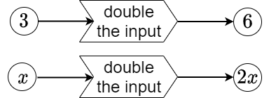
Example of a mathematical function The following two pictures with specific inputs show how the function machine with the rule "double the input" works:
The prescription in this function machine can be cast in a formula-like form and given a name as follows:
When inputting the number \(3\), this function machine returns the number \(6\) as output. Any input, say \(x\), yields the output \(2x\). In other words \(f(3)=6\) and \(f(x)=2x\). Mathematicians would rather stick the definition \(f(x)=2x\) as a label on the machine. The mathematical notation \(f: x\mapsto 2x\) resembles the way this function can be defined in R:
> f <- function(x) { 2*x }
> f(3)
[1] 6
Example of a mathematical algorithm A function in R does not have to be a mathematical function. Sometimes it is just an algorithm to compute a value. For example, the function \(e^x\) has the following power series expansion: \[\begin{aligned}e^x &= 1+x+\frac{x^2}{2!}+\frac{x^3}{3!}+\frac{x^4}{4!}+\cdots\\ &= \sum_{k=0}^{\infty}\frac{x^k}{k!}\end{aligned}\] Now suppose that we give polynomial functions \(F_n(x)\) ) as function statement the polynomial that you would get when you cut off the power series after \(n\) terms. So: \[F_n(x)=\sum_{k=0}^{n}\frac{x^k}{k!}\] In this way we get a series of functions \(F_1, F_2, \cdots\) Since we do not want to define each function separately, we construct an R function F with two arguments, namely \(n\) and \(x\):
F <- function(n, x) {
       sum_of_numbers <- 0
       for (k in 0:n) {
         sum_of_numbers <- sum_of_numbers + x^k/factorial(k)
       }
       return(sum_of_numbers)
     }
print(F(3, 1))   # rough approximation of the number e
print(F(10, 1))  # good approximation of the number e
print(F(100, 1)) # even better approximation of the number e
You get three number as output, viz. 2.66667, 2.716667, and 2.718282 The last two instructions show that the function for \(n=10\) and \(x=1\) returns a numerical result that approximates the exact value of \(e\), the base of the natural logarithm, to an accuracy of 6 decimal places. The deviation of the series approximation from the exact value is called truncation error of the approximation.
Example of a function with user interaction and side effects Functions in R can be versatile in nature. For example, they can have side effect like printing a message or plotting a graph, or you can have interactivity, meaning that there is a human operator to interact with the function, for example provide input for the instructions to be carried out.
As an example we show an R script in which a function is defined that asks its user for three positive real numbers and then checks if a triangle exists with the three number entered as lengths of the edges. In both cases, an appropriate message is printed, and whenever such a triangle exists, a sample triangle is drawn. Note that three positive real numbers allow the creation of a triangle with the requested lengths of sides if and only if the sum of any pair ofspecified numbers is greater than the other specified number.
Suppose, you have an R file named triangle.R in the directory C:/temp on an MS WIndows computer that contains the following script:
sides_of_triangle_Q <- function() {
 p <- as.numeric(readline(prompt = 'Enter a positive real number p = '))
 q <- as.numeric(readline(prompt = 'Enter a positive real number q = '))
 r <- as.numeric(readline(prompt = 'Enter a positive real number r = '))
 if (p > 0 & q > 0 & r > 0 & p < (q + r) & q < (r + p) & r < (p + q)) {
 print("A triangle with requested lengths of edges is possible.")
 x <- (q^2 + r^2 - p^2) / (2*r)
 y <- sqrt(2*p^2*(q^2 + r^2) -(q^2-r^2)^2 - p^4) / (2*r)
 plot(c(0,r,x,0), c(0,0,y,0), type="l", lwd=3, xlab="", ylab="", asp=1)
 } else {
 print("No triangle with requested lengths of edges is possible.")
 }
}

if(interactive()) sides_of_triangle_Q()
When you enter the instruction source("C:/temp/triangle.R") in the console, then you will be prompted to enter three positive real numbers. In the session below, the result is a message that there does not exist a triangle with lengths 1, 2, and 3 for edges.
> source("C:/temp/triangle.R")
Enter a positive real number p = 3
Enter a positive real number q = 2
Enter a positive real number r = 1
[1] "No triangle with requested lengths of edges is possible."
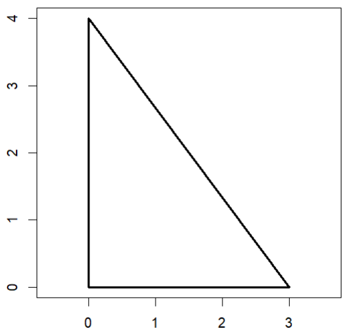
When you redo this source instruction and enter the numbers 3, 4, and 5 as possible lengths of edge of a triangle when prompted, thenyou get the confirmation that this is possible and a triangle matching the conditions is drawn.
> source("C:/temp/triangle.R")
Enter a positive real number p = 5
Enter a positive real number q = 4
Enter a positive real number r = 3
[1] "A triangle with requested lengths of edges is possible."


