Changing the margins Maybe you noticed that without a title of subtitle, the margins around a plot are quite large. The reason is that a single plot in R, known as a figure, comprises a plot region surrounded by margins (possibly containing axis labels, titles, etc.) and (usually) bounded by the axes themselves. See the figure below where tow optional arguments are shown to specify the margins.

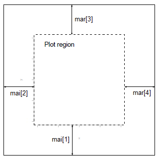
You can specify the size of the margins in a plotting function such as plot() via

• mai = c(s1, s2, s3, s4), where s₁, s₂, s₃, and s₄ are the sizes of the bottom, left, top and right margins, respectively, measured in inches;
• mar = c(s1, s2, s3, s4), where s₁, s₂, s₃, and s₄ are the sizes of the bottom, left, top and right margins, respectively, measured in the number of text lines. See the figure below.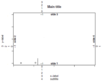
  
  

The default margin sizes are just over 5, 4, 4, and 2 text lines. You might set par(mar=c(4,4,2,2)+0.1) before plotting. This shaves one line off the bottom margin and two lines off the top margin of the plot, which will reduce the amount of unused whitespace when there is no main title or subtitle for subsequent plots.

Setting the size of the plot window Sometimes the plot window in RStudio is a bit small, or does not have the right dimensions for the type of plot that you need. In those cases you may want to use the function windows( ) on MS Windows computers or quartz( ) on computer running the MacOS system. The useful input arguments to these commands are the width = ... and height = ... options. The input to these options need to be specified in inches.

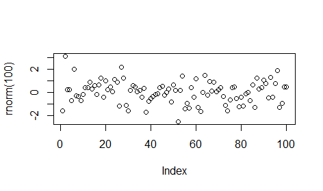
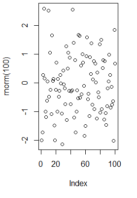
Let's create two windows to illustrate this: a first window of 5 inches wide and 3 high, and a second of 3 inches high and 5 wide. The outputs are shown below.

windows(width=5, height=3) # or on MacOS:  quartz(width=5, height=3)
plot(rnorm(100))
				
windows(width=3, height=5) # or on MacOS:  quartz(width=3, height=5)
plot(rnorm(100))

Saving an image If you're running R through Rstudio, then the easiest way to save your image is to click on the "Export" button in the Plot panel. When you do that you'll see a menu that contains the options "Save Plot as PDF" and "Save Plot as
Image". Both will bring up dialog boxes that give you a few options that you can play with, but besides that it's pretty simple.

Alternatively, you can use a command-sequence for saving a figure to a file. It similar to the saving of data, but instead of the function write.table(), you will use the functions pdf(), png(), svg(), jpeg(), tiff(), postscript(), and so on., depending on the type of desired output. In general the pdf, png and svg formats are the best graphical formats to use.

As an example, to save a figure to a pdf file file we use the following R script:

setwd("C:/temp")
pdf(file = ".example_scatter.pdf")
plot(rnorm(100))
dev.off()

1. The function setwd() sets the working directory where the pdf file can be found afterwards;
2. The function pdf() tells R to open a pdf file, and write the output of a plot or plots.
3. Plotting commands (the same ones you would normally use to get them on the screen) are given.
4. The instruction dev.off( ) tells R to close the pdf file (a 'device'), and return the plotting to the R console or the RStudio plot panel.

Enter ?pdf and ?png in the R console for more info. If you want to know which output formats ('devices' in programmer's jargon) are available use ?devices.

Sometimes you may have opened so many figure windows in R that it becomes hard to keep an overview. To see the list of all open devices use the function dev.list(). To close all devices, not only the last one, use graphics.off().