1. Descriptive Statistics: Practical 1
 Measures of Central Tendency
R contains the commands mean()and median() to calculate exactly these statistics based on data. If you want to visualise the complete distribution, you can check the frequency distribution with the command hist(). This will create a histogram in the lower-right pane (the Plots Tab).
Let's have a look at these functions.
The mean of lifeExp for 1967 #=# #55.68#
Calculating the mean of lifeExp for the whole dataframe is simply done with:
mean(G$lifeExp)The frequency distribution can be visualised with the command:
hist(G$lifeExp)
If you want to calculate the mean for only 1967, you can first make a subset of the data with:
G1967 <- G[G$year == 1967,]after which you apply the function for mean on the lifeExp.
mean(G1967$lifeExp)Alternatively, you can do this also in one line by selecting all the rows in which the year is 1967 and selecting the column 'lifeExp'. Apply the mean to this selection.
mean(G[G$year == 1967, 'lifeExp'])
Or by selecting the column 'lifeExp' and subsequently all the rows in which the year is 1967:
mean(G$lifeExp[G$year == 1967])
The mode is the value that has highest number of occurrences in a set of data. Unike mean and median, mode can have both numeric and character data, however it is usually not giving insightfull results for continuous numeric data (sometimes it is relevant for discrete data).
R does not contain a separate command to calculate the mode. But there is a more general command that does provide the mode as output as well, table(). The table() command counts the number of occurrences to each category in a variable or, in other words, it makes a frequency table. It should only be applied to a vector with categorical data (which could be stored as character strings, but also as integers).
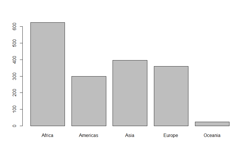
table() to calculate the frequency distribution for the variable continent. Store the results in an object CF. Think about the values that are shown, what do they mean? Based on this data, what would be the mode for the variable continent?
CF <- table(G$continent)
The table shows the number of observations in the dataframe per continent. As the dataframe contains multiple years, this does not correspond to the number of countries per continent! The mode for the variable continent is Africa. You can also visualise this in a barchart with the following comment:
barplot(CF)
(In case you are wondering how to find the number of countries per continent, remember the functions
length() and unique()! e.g. length(unique(G[G$continent == 'Europe', 'country'])) gives the number of unique countries in Europe).Quantiles specify where specific fractions of the data are located. The 50th quantile is in fact the median. The function quantile() gives quantiles in R.
The 70th quantile of lifeExp for Africa #=# #52.73#
Use the help function:
?quantile if you need help to specify the right input arguments to this function. Here you can read that you can specify the quantile with a probability vector in the range 0 to 1. That means that we need to specify 0.7 for the 70th quantile.
quantile(G$lifeExp, 0.7)
We can calculate the same quantile for only Africa by first making a subset with only data for this content.
G_Africa <- G[G$continent == 'Africa', ]Then we can calculate the 70th quantile:
quantile(G_Africa$lifeExp, 0.7)
Alternatively, you could do this in one line by specifying the rows with only the continent selected and the column lifeExp. Then apply the
quantile() function. quantile(G[G$continent == 'Africa', 'lifeExp'], 0.7)


