4. Probability Distributions: Probability Models
 Continuous Probability Models
Continuous Probability Model
If the sample space #\Omega# of a random experiment consists of an uncountable set of outcomes, we must use a continuous probability model to assign probabilities to events.
Intervals are examples of uncountable sets. For example the interval #(0, \infty)# or the interval #[1,5]#.
Density Curve
The graph of a continuous probability model is called a density curve, and has the following properties:
- A density curve is always on or above the horizontal axis.
- The total area under the whole density curve always equals #1#.
Continuous Model: Calculating the Probability of an Event
For a continuous probability model, the probability of an event is the area under the density curve above all outcomes in that event.

Let #X# denote a number randomly generated from the interval #[0, 5]#.
Calculate the probabilities of the following events:
- #A = \{"\text{number}\gt 3"\}#
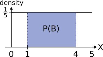
- #B = \{"\text{number between } 1 \text{ and }4"\}#
Since all numbers in the interval #[0,5]# have an equal chance of selection, the density curve is flat:

It is a rectangle with a width of #5#. This means that its height must be #\frac{1}{5}#, since the total area under the density curve has to equal #1#:
\[5\cdot x = 1 \Rightarrow x = \cfrac{1}{5}\]
The probability of event #A# is:
| \[\mathbb{P}(A)=(5-3)\cdot \cfrac{1}{5}=\cfrac{2}{5}\] |
 |
The probability of event #B# is:
| \[\mathbb{P}(B)=(4-1)\cdot \cfrac{1}{5}=\cfrac{3}{5}\] |
 |


