4. Probability Distributions: Practical 4
 Normal random variables
The normal distribution is the most widely used distribution in statistics. Its shape is determined by two parameters: the mean and standard deviation. The common way to specify that a random variable #X# has a normal distribution with a mean #10# and standard deviation #3# is as follows
#X \sim N(10,3)#.
We will apply this notation throughout this text.
Probability density
The probability density of a given value of #x# and a given normal distribution #N(\mu,\sigma)#, can be calculated with the function dnorm(x, mean, sd). Probability density plots are a nice way to visualise the probability densities associated with a given normal distribution.
Create a probability density plot of a normal distribution #N(0,1)#.
?seq).x <- seq(-6, 6, 0.01)Now you can use the
dnorm() function to calculate the probability density at each of these values of #x# (#P(X = x)#) for the specified normal distribution. These will be your y-values.y <- dnorm(x, mean=0, sd=1)
The last step is the actually plotting. Here, we used the parameter option
type='l' to specifies that a line should be plotted rather than e.g. points. Mind that the 'l' in the code below stands for the lowercase letter L and not the number 1.plot(x=x, y=y, type='l')
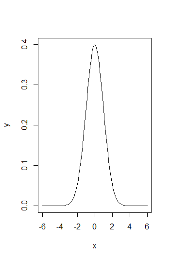
In the resulting plot, you see that the probability density is largest at the mean. It is furthermore symmetrical around the mean, thus for a random variable #X \sim N(0,1)#, #P(X \leq -1) = P(X \geq 1)#.
In the example below, we create a probality density plot of a normal distribution #N(0,2)#.
Now calculate values for normal distribution #N(0,2)# and plot these in the same figure, to see what a distribution with the same mean but larger standard deviation looks like.
You can use the same x-values as in the previous example. So you only need to calculate the new y-values, which are again the probability densities at each of these values of x (#P(X = x)#). This time for the normal distribution #N(0,2)#.
y <- dnorm(x, mean=0, sd=2)
The lines() command adds a line to a plot that already exist (without changing the ranges of the axes or adjusting anything that already exists in the plot).
lines(x, y, col='red')
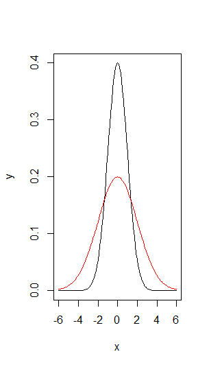
The result shows a curve that has a lower peak but stretches all the way from #-6# to #6# before the y-values get close to zero. This can be explained again with the empirical rule stating that #99.7\%# of scores will be located within #3# standard deviations from the mean.
Cumulative probability density
To answer real-life questions about a random variable, we need to turn probability densities into probabilities. This means we are not looking at the height of the probability density curve, but rather the surface under the curve. A typical example of such a question is:
If the air temperature at 12:00 in Amsterdam in March is normally distributed with a mean of #10# degrees C and a standard deviation of #4# degrees, what is then the probability to experience a day where it is freezing (i.e. a temperature of #0# degrees or less) at noon?
To answer such a question, we would consider #X \sim N(10,4)# and find the value #P(X \le 0)#.
The cumulative probability density function calculates the values #P(X \le x)#. In mathematical terms: the cumulative probability density function integrates (=sums) the probability density values from #-\inf# up to the value #x#.
The command which calculates cumulative probability densities for a normal variable is pnorm(x, mean, sd).
Create a cumulative probability density plot for the normal distributions #N(0,1)# and #N(0,2)#.
x <- seq(-6, 6, 0.01)Now you use the
pnorm() function to calculate the cumulative probability density at each of these values of x (#P(X \le x)#) for the specified normal distributions. These will be your y-values.cp1 <- pnorm(x, mean=0, sd=1)Once, you have calculated the x- and y-values, you are ready for plotting!
cp2 <- pnorm(x, mean=0, sd=2)
plot(x=x, y=cp1, type='l')
lines(x=x, y=cp2, col='red')
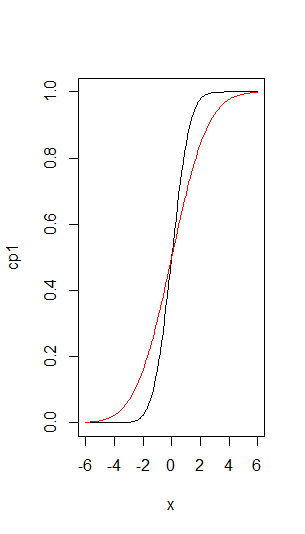
As can you see, the cumulative probability goes up from #0# to #1# when we go from small values of #x# to large values. And for the distribution with a smaller #\sigma# (in black) the curve is a lot steeper (but starting to increment also a lot later) than with the larger #\sigma# (in red).
Let's assume you want to know the cumulative probability #P(X \le -1)# for the variable #X \sim N(0,1)#. You then use the following command to find this value.
pnorm(-1, mean=0, sd=1)
If instead, you want to know the probability #P(X > -1)#, you can calculate #1 - P(X \le -1)# or use the fourth input argument in the pnorm() command: lower.tail=FALSE.
1 - pnorm(-1, mean=0, sd=1)
is the same as:
pnorm(-1, mean=0, sd=1, lower.tail=FALSE)
Suppose you have a variable #X \sim N(0,0.2)#. Calculate for this variable the probability #P(X \le 0)#. Round your answer to 3 decimal points and check your answer visually with a cumulative probability plot.
To calculate the cumulative probability #P(X \le 0)#, you should use the function
pnorm(x, mean, sd):pnorm(0, mean=0, sd=0.2)
To check this answer visually you can create a cumulative probability plot. First create a sequence of x-values, ranging from #\mu - 3* \sigma# to #\mu + 3* \sigma# to ensure that the complete sigmoid is visualized.
x <- seq(-0.6, 0.6, 0.01)Next, calculate the cumulative probability for all x-values using again the
pnorm() function and plot the result against the x-values.cp <- pnorm(x, mean=0, sd=0.2)In the resulting plot, you can find the #x=0# to confirm your result.
plot(x=x, y=cp, type='l')
Inverse Cumulative Probability Density
Another type of real-life questions about a random variable regards exactly the opposite from what is provided by the cumulative probability density: we would like to choose a value for #X# so that the chance that #X# stays below this value is equal to the specified probability value. Consider for example this question:
The yearly extreme water level at a certain location has a mean #+4# m NAP with a standard deviation of #1# m. What should the height of the dyke be at that location if we want to have a probability of flooding in less than #1# out of #1000# years?
The mathematical formulation would be: for a random variable #X \sim N(4,1)#, what is the value of #q# such that for #P(X \leq q) = 0.001#?
The function we need is doing the opposite from the cumulative probability density and in mathematics the term for this is the inverse. Applying an inverse function means that if you would have a function F() which uses the input x to calculate an output y, then the inverse function Fi() would take y as input to calculate an output x.
The function qnorm()is the inverse function of pnorm(), it calculates the inverse cumulative probability density function.
Create an inverse cumulative probability density plot for the normal distributions #N(0,1)# and #N(0,2)#.
p <- seq(0, 1, 0.01)Now you use the
qnorm() function to calculate the corresponding values of #X#.q1 <- qnorm(p, mean=0, sd=1)At this point, you can plot both distributions.
q2 <- qnorm(p, mean=0, sd=2)
plot(x=p, y=q1, type='l', ylim=c(-6,6))
lines(x=p, y=q2, col='red')
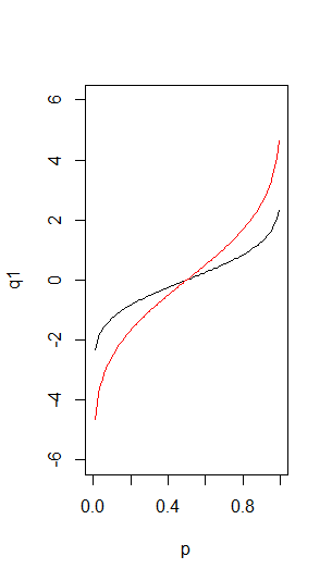
As you see, this plot shows the values of #X# corresponding to the probability #p# for the two distributions.
Suppose you have a variable #X \sim N(5,1)#. Calculate for this variable the value of #q# such that for #P(X \leq q) = 0.58#.
Round your answer to 3 decimal points and check your answer visually with an inverse cumulative probability plot.
To calculate the value of #q# such that for #P(X \leq q) = 0.58#, you should use the function
qnorm(p, mean, sd):qnorm(0.58, mean=5, sd=1)
To check this answer visually you can create an inverse cumulative probability plot. First create a sequence of p-values, ranging from #0# to #1#.
p <- seq(0, 1, 0.01)Next, calculate the inverse cumulative probability for all p-values using again the
qnorm() function and plot the result against the p-values.q <- qnorm(p, mean=5, sd=1)In the resulting plot, you can find the value of #q# for which the probability is #0.58# to confirm your result.
plot(x=p, y=q, type='l')


