The binomial distribution is the distribution that describes the number of successful outcomes from a sequence of independent experiments with two possible outcomes (like flipping a coin, which would give either heads or tails). This distribution has two parameters: 1) the number of experiments that are conducted and 2) the probability to get a successful outcome for a single experiment.

Let's consider two concrete examples.

If you flip a coin $10$ times, then the number of times you get 'heads' has a binomial distribution. Coins will have a probability of $0.5$ to give heads. So most times you will just get $5$ times 'heads', and occasionally the number of heads will be very low (like $0$ or $1$ time) or high ($8$ or $9$ times).

The exams for some courses are in the form of 'multiple choice' questions. Let's consider the case that you would have to take an exam with $20$ MC questions which each has $4$ options. In an extreme case where you wouldn't have learned anything and just filled-in your answers randomly. What would then be the chance to pass the exam with $11$ correct answers? In this example, the number of correct answers has a binomial distribution and through the binomial distribution, you can calculate the probability of passing the exam by pure guesswork.

A binomial random variable is discrete since it can only take on positive integer values ($0$, $1$, $2$, etc.). Note that this is different from a normally distributed random variable which is continuous and can take on any real value ($-0.231$, $4.26$, etc.). If a probability distribution is discrete, then the probability density function is called a probability mass function, because it does give actual probabilities to get a specific outcome for the binomial random variable.

The commands in R for the binomial distribution for a random variable $X$ are:

• dbinom() - to calculate the probability that you get exactly $x$ successes (in $n$ experiments, where the theoretical probability of success is $p$)
• pbinom() - to calculate the probability that the number of successes is within a given interval
• qbinom() - to calculate threshold values for the number of successes that will be exceeded with a given probability

The common way to specify that a random variable $X$ has a binomial distribution, based on $10$ experiments, with a theoretical probability of success of $0.5$ is as follows.

$X \sim B(10,0.5)$

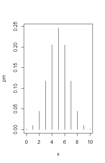
The following example illustrates how the distribution (the probability mass function) of a random variable $X \sim B(10,0.5)$ can be plotted.

First, you have to generate a sequence of values that you will use as x-values for the plot, as you did with the plots for the normal distribution. However, as the values of the binomial distribution are discrete, the sequence should contain only positive integers.

x <- 0:10

Now you can use the dbinom() function to calculate the probability mass at each of these values of $x$ ($P(X = x)$) for the specified binomial distribution. These will be your y-values.

y <- dbinom(x, size=10, prob=0.5)

The last step is the actual plotting. Here, we used the parameter option type='h' to specify that vertical bars should be plotted at each of the values for x (like a barplot, but then only with bars at the allowable x-values).

plot(x=x, y=y, type='h')

New example

You can use the same sequence of values for the x-axis as you did in the previous example. If you still have the x-values stored in R's working environment, there is no need to rerun the command.

x <- 1:10

Now you use the pbinom() function to calculate the cumulative probability at each of these values of $x$ ($P(X \le x)$) for the specified binomial distributions. These will be your y-values.

cp <- pbinom(x, size=10, prob=0.5)

Once, you have calculated the x- and y-values, you are ready for plotting!

plot(x=x, y=cp, type='s')

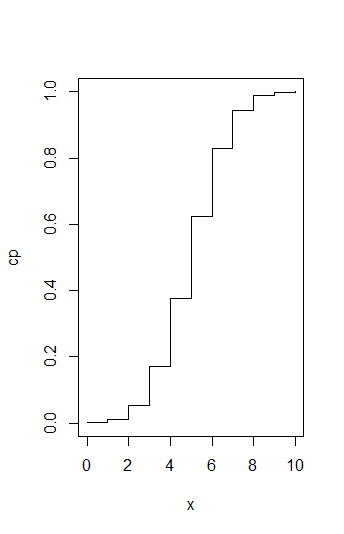
In this graph, the parameter option type='s' states that the data should be plotted as a 'staircase plot'. The probabilities add-up in a stepwise fashion. In general, for discrete probability distributions, you would need to specify the plotting options type='h' and type='s' for the probability mass and cumulative probability plots respectively.

New example