5. Sampling: Sampling Distributions
 Sampling Distribution of the Sample Proportion
A type of variable which is commonly studied in statistics is the binary variable.
#\phantom{0}#
Binary Variable
Definition
A binary or dichotomous variable is a categorical variable that can only take on #2# possible values.
Examples
- True/false
- Success/failure
- Yes/no
- On/off
#\phantom{0}#
The mean of a binary variable is mathematically equivalent to the proportion.
#\phantom{0}#
Proportion
Definition
In statistics, a proportion refers to the fraction of a group that possesses a particular characteristic.
The population and sample proportion are denoted #\pi# and #\hat{p}#, respectively.
Formula
#\text{proportion}=\cfrac{\text{# of individuals with characterstic}}{\text{total number of individuals}}#
#\phantom{0}#
When using a sample proportion to estimate a population proportion, the sampling distribution of the sample proportion can be used to determine how much estimation error is reasonable to expect.
#\phantom{0}#
Sampling Distribution of the Sample Proportion
The sampling distribution of the sample proportion is the probability distribution of the sample proportions of every possible sample of a particular size #n# that can be drawn from a population.
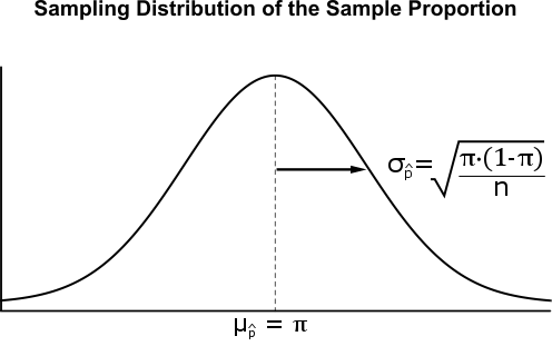
The mean of the distribution of sample proportions is called the expected value of the sample proportion and is denoted #\mu_{\hat{p}}#.
The standard deviation of the distribution of sample proportions is called the standard error of the sample proportion and is denoted #\sigma_{\hat{p}}#. The standard error is a measure of how much discrepancy to expect between a sample proportion #\hat{p}# and the population proportion #\pi#.
Conditions for Normality
For any population of which a proportion #\pi# possesses a particular characteristic, the sampling distribution of the sample proportion for samples of size #n# may be considered approximately normal if both of the following conditions are satisfied:
- We expect there to be at least #10# positive cases: #n \cdot \pi \geq 10#
- We expect there to be at least #10# negative cases: #n \cdot (1-\pi) \geq 10#
If both these conditions are satisfied, the sampling distribution of the sample proportions may be considered approximately normal with parameters:
- #\mu_{\hat{p}}=\pi#
- #\sigma_{\hat{p}}=\sqrt{\cfrac{\pi \cdot(1-\pi)}{n}}#
\[\hat{p} \sim N(\pi, \sqrt{\cfrac{\pi \cdot (1-\pi)}{n}})\]

#\mu_{\hat{p}} = 0.10#
Investigate whether the sampling distribution of the sample proportion may be considered approximately normal:
- #n\cdot \pi = 110 \cdot 0.10 = 11 \geq 10#
- #n\cdot (1-\pi) = 110 \cdot (1-0.10) = 99 \geq 10#
Since both conditions are satisfied, the expected value of the sample proportion, #\mu_{\hat{p}}#, is equal to the population proportion #\pi#:
\[\mu_{\hat{p}} = \pi= 0.10\]


