7. Hypothesis Testing: Introduction to Hypothesis Testing
 Setting the Criteria for a Decision
Once the hypotheses of the test have been formulated, the next step is to set the criteria for a decision. This should always be done before the sample data is collected.
Specifically, we need to determine what values of the sample statistic will lead to the rejection of the null hypothesis. Because a sample provides an incomplete picture of a population, some discrepancy between a sample statistic and its corresponding population parameter is to be expected.
How much discrepancy is reasonable to expect can be derived from the sampling distribution of the sample statistic under the null hypothesis. If the null hypothesis is true, it is likely that the sample statistic will be relatively close in value to the mean of the sampling distribution.
As the difference between a sample statistic and the mean of the hypothesized sampling distribution increases, your confidence in the null hypothesis being true should decrease. If you observe a sample statistic that is extremely unlikely to occur given that the null hypothesis is true, this should lead to the rejection of the null hypothesis. In order to formalize what constitutes as an extremely unlikely result, the significance level of the test needs to be set.
#\phantom{0}#
Significance Level and Critical Values
The significance level, denoted #\alpha#, of a statistical test is the probability threshold that determines how unlikely a sample statistic has to be in order for the null hypothesis #H_0# to be rejected.
The range of values for the sample statistic that will lead to the rejection of the null hypothesis is called the critical region.
The boundary values of the critical region are called critical values.
Decreasing the significance level shrinks the critical region of the sampling distribution, meaning a smaller range of values will lead to the rejection of #H_0#.
Increasing the significance level expands the critical region of the sampling distribution, meaning a larger range of values will lead to the rejection of #H_0#.
Example of Setting Alpha
Setting an #\alpha = 0.05# significance level means that if you observe a sample statistic that has less than or equal to #5\%# chance of occurring if the null hypothesis is true, the null hypothesis should be rejected.
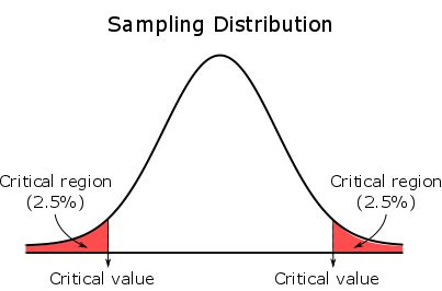
For a two-tailed test, the critical region is evenly split between both tails.
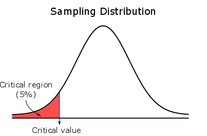
For a left-tailed test, the entire critical region is located in the left tail.
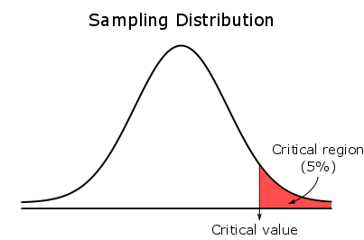
For a right-tailed test, the entire critical region is located in the right tail.
Choosing an Appropriate Significance Level
Note that the choice of the significance level #\alpha# should be made with care. The more consequential the acceptance of the alternative hypothesis, the smaller #\alpha# should be (for instance a murder trial, where the alternative hypothesis is that someone is guilty).
For example, #H_a: \mu \gt \mu_0# is a stronger hypothesis than #H_a: \mu \neq \mu_0#, because the former hypothesis not only specifies that #\mu# is different from #\mu_0# but also that #\mu# differs from #\mu_0# in a specific direction. So a smaller #\alpha# should be used for a one-tailed test than what is used for a two-tailed test.
An additional consideration is the severity of the consequences if a conclusion is made in favor of #H_a#, but this decision turns out to be a mistake. If severe harm could be caused (e.g. damage to someone's health, loss of large sums of money), then a smaller #\alpha# should be used.
On the other hand, using an #\alpha# that is too small could also have severe consequences, because concluding in favor of #H_0# when #H_a# is actually true might, for example, lead to the failure to provide a treatment for an illness that would have been effective.
#\phantom{0}#
When conducting a #z#-test, the Standard Normal Table is used to determine the boundaries of the critical region. For a #z#-test, the exact location of the boundaries is determined entirely by the alpha level of the test. The table below displays the most commonly used significance levels and the corresponding critical values.
\[\begin{array}{c|c}
\alpha&\text{Critical }z \text{ values}\\
\hline
0.10&\pm 1.645\\
0.05&\pm 1.96\\
0.01&\pm 2.58\\
\end{array}\]
3. Example Summer Course: Critical Region
If the null hypothesis is true, the Summer Course should have no effect on the students' grades and the population of students that participate in the Summer Course will be identical to that of the original population of students; that is, a normal distribution with #\mu = 6.5# and #\sigma=1#.
Next, it is needed to consider all possible outcomes for a sample of #n =100# students. This is the distribution of sample means for #n=100#. If the null hypothesis is true, then the distribution of sample means will have the following properties:
#\phantom{0}#
- #\mu_{\bar{X}}= \mu_0 = 6.5#
- #\sigma_{\bar{X}} = \cfrac{\sigma}{\sqrt{n}}=\cfrac{1}{\sqrt{100}} = 0.1#

Finally, the distribution of sample means is used to determine the critical region of the test. The university decides to set the alpha level of the test at #\alpha = 0.05#, meaning the critical region consists of the extreme #5\%# of the sampling distribution.
The critical values for a #z#-test with #\alpha =0.05# are #z = \pm 1.96#. This means that finding a #z#-statistic less than #-1.96# or greater than #1.96# should lead to the rejection of the null hypothesis.


