The value of #1.96# that was used in the previous paragraphs to calculate the 95% confidence interval was conveniently provided. But we can calculate this value based on our knowledge about probability distributions (see Chapter 4).

Let's see where this value comes from and also how it changes if the confidence level is set to another value.

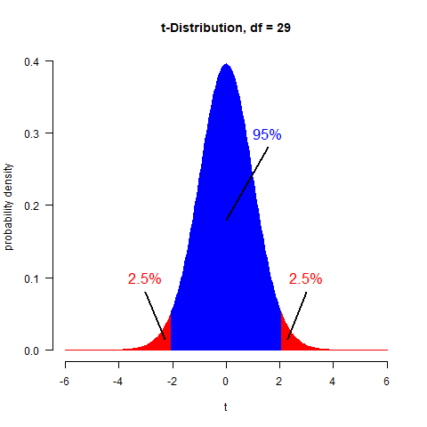
The value #1.96# is an approximation of the threshold value of a random variable #X# with t-distribution such that on average #0.95# of the observed values #x# will fall in the range #-1.96# to #1.96# (see the figure below).

The t-distribution is the distribution of a sample mean in the situation where you don't know the population standard deviation (which is almost always the case). In this situation you need to estimate both the population mean and the population standard deviation from the sample.

The shape of the t-distribution is very similar to the standard normal distribution (the z-distribution). In contrast to the z-distribution, which has no parameters, the t-distribution has 1 parameter, called 'degrees of freedom'. The value for this parameter is the sample size minus 1 (#df = n-1#).

In R, the following four probability-functions relate to the t-distribution (in this example based on a sample of size #30#).

dt(x=-3:3, df=29)     # probability densities for x = -3 ... 3
pt(q=-3:3, df=29)     # cumulative probability for x = -3 ... 3
qt(p=0.1,  df=29)     # critical value (X) such that P(t<X)=0.1
rt(100, df=29)        # generate 100 random values X ~ t(29)

The confidence interval of 95% that we have been using so far was referring to a probability level of #0.95#. But fact that the range #-1.96# to #1.96# (see the figure above) is centered around #0# implies that 2.5% of the values #x# are higher than #1.96#, and 2.5% of the values are lower than #-1.96#. So, to calculate the threshold value of #1.96# (or #-1.96#) we should not calculate

qt(p=0.95, df=29) ...

But rather

qt(p=0.975, df=29)    # P(t <=  2.045) = 0.975
qt(p=0.025, df=29)    # P(t <= -2.045) = 0.025

If you don't find the choice for the values of p intuitive, you can apply the following general calculation rule to obtain these based on the confidence interval (CI): #p_{up} = (100+CI)/200# and #p_{low} = 1 - p_{up} = (100-CI)/200#

p_low = (100 - 80)/200
p_up = (100 + 80)/200

qt(p=0.90, df=39)    # P(t <=  1.3036) = 0.90  
qt(p=0.10, df=39)    # P(t <= -1.3036) = 0.10

The threshold values that are calculated in this way are called #t# values. The probability level to which a #t# value relates is added as sub-script for clarity: # t_{0.1}=-1.299# and #t_{0.975}=2.045#

To summarize: the function qt() is used to calculate threshold values (#t# values) for a random variable of interest. The probability level chosen for this calculation follows from the confidence interval, by #p_{up} = (100+CI)/200#

The values at the x-axis of a #t# distribution (just as with the #z# distribution) are given in the units of 'standard deviations'. This means that a value of #2.045# should be understood as: '#2.045# standard deviations higher than the mean'.

This special meaning makes that the #t# values (threshold values for the t distribution) can be directly used for confidence intervals of other normally distributed variables as well, by multiplying the #t# value with the standard deviation for the variable of interest.

And this is exactly what we did in the previous paragraph to obtain the lower and upper coinfidence limits by:

#CL_{low} = \bar{x} - 2.045 * s / \sqrt{n}#

#CL_{up} = \bar{x} + 2.045 * s / \sqrt{n}#

set.seed(25)
samp = sample(V$ capaciteit, 50)

tval <- qt(p=(100+95)/200, df=50-1)

CL_low <- mean(samp) - tval*sd(samp)/sqrt(50)
CL_up <- mean(samp) + tval*sd(samp)/sqrt(50)