In the previous step, you used the linear model to predict the wish to move for new neighbourhoods based on the quality of life value. However, the linear model is based on some assumptions and the results of the predictions are only reliable if these assumptions hold. In addition, the results of the hypothesis tests (i.e. the p-value and associated conclusion about the linear relation between predictor and response variable) are only valid if the model assumptions hold.

Let's therefore, check the assumptions of linear regression: 1) linearity, 2) homoscedasticity, 3) normality of residuals and 4) absence of influential datapoints.

1) Linearity

Recall that before you started the linear regression, you checked if the relation between quality of life and wish to move was approximately linear with a scatterplot. If that was the case, the residuals (the difference between each observed point and the predicted value) of the regression should show no apparent pattern. The residuals can conveniently be extracted from the model object m1 with the function residuals()

residuals(m1)

The plot of predicted values for the response variable against the residuals provides a very good first check for a pattern in the residuals.

plot(predict(m1), residuals(m1))

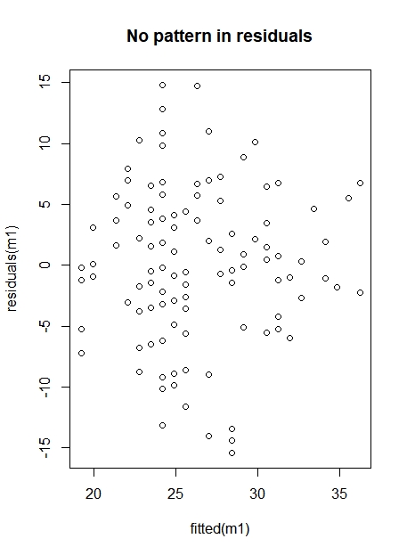
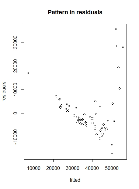
In this case, there is no apparent pattern, and therefore there is no reason to believe that the linearity assumption is violated. Figure 3 shows two residual plots. The left illustrates a situation with no pattern in the residuals, at the right, however, there is a structural deviation around the y=0 line and in this case the fitted model is not reliable.

Figure 3. Residuals plot with (right) and without (left) pattern in the residuals.

2) Homoscedasticity

The assumption of homoscedasticity is met if the variance of your data is approximately equal across the range of your predicted values. If you have changing variance, this is called heteroscedasticity. For the homoscedasticity assumption to be met, the residuals of your model need to roughly have a similar amount of deviation from your predicted values. This assumption can be checked with the residuals plot we already made.

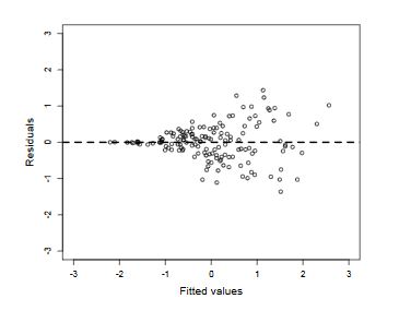
In our case, you see that the variance of the higher values is slightly decreasing (Figure 3, left). However, we have very few points with high values, so this is not a problem. In general, a residuals plot is good when the residuals (errors) are random and the residuals plot looks somewhat blob-like. An example of a residuals plot that shows clear heteroscedasticity (and the linear model is for that reason problematic) is shown in Figure 4.

Figure 4. Heteroscedasticity

3) Normality of residuals

In addition to linearity and homoscedasticity, the residuals have to be checked on normality. We will check this through a histogram.

hist(residuals(m1))

The distribution of the residuals is not perfectly normal, but this is close enough to be considered normal. In general, the assumption of normality of the residuals is the least important, especially with large data sets (use n>30 as a rule of thumb for linear regression with one predictor variable). So a small deviation is not problematic.

4) Absence of influential datapoints

The last assumption we are going to check is the absence of influential datapoints. Influential datapoints are points that substantially influence the regression line by "pulling the line towards them". The formal way to find them is by leaving a point out of the data set and evaluating how much the regression equation changes as a result of that. But usually influential datapoints can also be identified on the scatterplot of the model: an influential point is located at the outer ends of the predictor variable range, and is relatively isolated in the scatter plot. In our example there are no influential datapoints.

None of the four assumptions have been violated and therefore we can stand by the conclusions we did draw before.

Of course, the validity of this model doesn't say anything about other possible relations in the data. In the exercises, you will practice with the criminality index and see if that variable can explain the wish to move as well.